Essential commands

Essential commands#

The following describes essential commands for interacting with the AlphaGenome API. It is broken into two sections: data and methods.

Tip

Open this tutorial in Google colab for interactive viewing.

# @title Install AlphaGenome

# @markdown Run this cell to install AlphaGenome.
from IPython.display import clear_output
! pip install alphagenome
clear_output()

Imports#

from alphagenome.data import genome
from alphagenome.models import dna_client
import numpy as np
import pandas as pd
from google.colab import userdata

Data: model inputs#

Genomic interval#

A genomic interval is specified using genome.Interval:

interval = genome.Interval(chromosome='chr1', start=1_000, end=1_010)

By default, these are human hg38 intervals. See the FAQ for more details on organisms and genome versions.

Interval properties#

Access some handy properties of the interval:

interval.center()

interval.width

Resize#

Use genome.Interval.resize to resize the interval around its center point:

interval.resize(100)

Interval(chromosome='chr1', start=955, end=1055, strand='.', name='')

Compare intervals#

We can also check the interval’s relationship to other intervals:

second_interval = genome.Interval(chromosome='chr1', start=1_005, end=1_015)

interval.overlaps(second_interval)

True

interval.contains(second_interval)

False

interval.intersect(second_interval)

Interval(chromosome='chr1', start=1005, end=1010, strand='.', name='')

As a subtle point, AlphaGenome classes use 0-based indexing, meaning that the interval includes the base pair at the start position up to the base pair at the end-1 position. See the FAQ for more on this topic.

Genomic variant#

A genome.Variant specifies a genetic variant:

variant = genome.Variant(
    chromosome='chr3', position=10_000, reference_bases='A', alternate_bases='C'
)

This variant changes the base A to a C at position 10_000 on chromosome 3. Note that the position attribute is 1-based to maintain compatibility with common public variant formats (see FAQ for more info.)

Insertions or deletions (indels)#

Variants can also be larger than a single base, such as insertions or deletions:

# Insertion variant.
variant = genome.Variant(
    chromosome='chr3',
    position=10_000,
    reference_bases='T',
    alternate_bases='CGTCAAT',
)

# Deletion variant.
variant = genome.Variant(
    chromosome='chr3',
    position=10_000,
    reference_bases='AGGGATC',
    alternate_bases='C',
)

The sequence we pass for the reference_bases argument could differ from what is actually at that location in the hg38 reference genome. The model will insert whatever is passed as the reference and alternate bases into the sequence and make predictions on them.

Reference interval#

We can get the genome.Interval corresponding to the reference bases of the variant using genome.Variant.reference_interval:

variant = genome.Variant(
    chromosome='chr3', position=10_000, reference_bases='A', alternate_bases='T'
)

variant.reference_interval

Interval(chromosome='chr3', start=9999, end=10000, strand='.', name='')

A common use-case is to make predictions in a genome region around a variant, which involves resizing the genome.Variant.reference_interval to a sequence length compatible with AlphaGenome:

input_interval = variant.reference_interval.resize(
    dna_client.SEQUENCE_LENGTH_1MB
)
input_interval.width

Overlap with interval#

We can also check if a variant’s reference or alternate alleles overlap an genome.Interval:

variant = genome.Variant(
    chromosome='chr3',
    position=10_000,
    reference_bases='T',
    alternate_bases='CGTCAAT',
)

interval = genome.Interval(chromosome='chr3', start=10_005, end=10_010)

print('Reference overlaps:', variant.reference_overlaps(interval))
print('Alternative overlaps:', variant.alternate_overlaps(interval))

Reference overlaps: False
Alternative overlaps: True

Data: model outputs#

Track data#

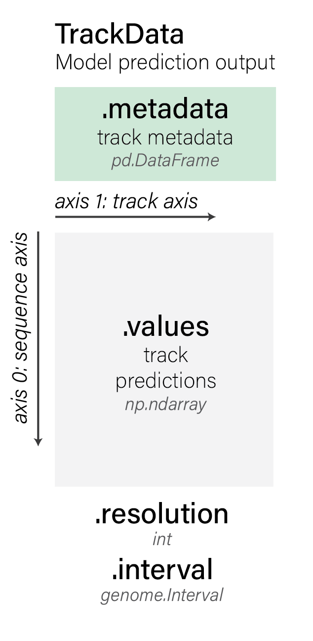
track_data.TrackData objects store model predictions. They have the following properties (using tdata as an example of a track_data.TrackData object):

tdata.values store track predictions as a numpy.ndarray .
tdata.metadata stores track metadata as a pandas.DataFrame. For each track in the predicted values, there will be a corresponding row in the track metadata describing its origin.
tdata.uns contains additional unstructured metadata as a dict.

From scratch#

You can create your own track_data.TrackData object from scratch by specifying the values and metadata manually. The metadata must contain at least the columns name (the names of the tracks) and strand (the strands of DNA that the tracks are on):

from alphagenome.data import track_data

# Array has shape (4,3) -> sequence is length 4 and there are 3 tracks.
values = np.array([[0, 1, 2], [3, 4, 5], [6, 7, 8], [9, 10, 11]]).astype(
    np.float32
)

# We have both the positive and negative strand values for track1, while track2
# contains unstranded data.
metadata = pd.DataFrame({
    'name': ['track1', 'track1', 'track2'],
    'strand': ['+', '-', '.'],
})

tdata = track_data.TrackData(values=values, metadata=metadata)

Resolution#

It’s also useful to specify the resolution of the tracks and the genomic interval that they come from, if you have this information available:

interval = genome.Interval(chromosome='chr1', start=1_000, end=1_004)

tdata = track_data.TrackData(
    values=values, metadata=metadata, resolution=1, interval=interval
)

Note that the length of the values has to match up with the interval width and resolution. Here is an example specifying that the values actually represent 128bp resolution tracks (i.e., each number is a summary over 128 base pairs of DNA):

interval = genome.Interval(chromosome='chr1', start=1_000, end=1_512)

tdata = track_data.TrackData(
    values=values, metadata=metadata, resolution=128, interval=interval
)

Converting between resolutions#

We can also interconvert between resolutions. For example, given 1bp resolution predictions, we can downsample the resolution (by summing adjacent values) and return a sequence of length 2:

interval = genome.Interval(chromosome='chr1', start=1_000, end=1_004)

tdata = track_data.TrackData(
    values=values, metadata=metadata, resolution=1, interval=interval
)

tdata = tdata.change_resolution(resolution=2)
tdata.values

array([[ 3.,  5.,  7.],
       [15., 17., 19.]], dtype=float32)

We can also upsample track data to get back to 1bp resolution and a sequence of length 4 by repeating values while preserving the sum:

tdata = tdata.change_resolution(resolution=1)
tdata.values

array([[1.5, 2.5, 3.5],
       [1.5, 2.5, 3.5],
       [7.5, 8.5, 9.5],
       [7.5, 8.5, 9.5]], dtype=float32)

Filtering#

track_data.TrackData objects can be filtered by the type of DNA strand the tracks are on:

print(
    'Positive strand tracks:',
    tdata.filter_to_positive_strand().metadata.name.values,
)
print(
    'Negative strand tracks:',
    tdata.filter_to_negative_strand().metadata.name.values,
)
print('Unstranded tracks:', tdata.filter_to_unstranded().metadata.name.values)

Positive strand tracks: ['track1']
Negative strand tracks: ['track1']
Unstranded tracks: ['track2']

Resizing#

We can resize the track_data.TrackData to be either smaller (by cropping):

# Re-instantiating the original trackdata.
tdata = track_data.TrackData(
    values=values, metadata=metadata, resolution=1, interval=interval
)

# Resize from width (sequence length) of 4 down to 2.
tdata.resize(width=2).values

array([[3., 4., 5.],
       [6., 7., 8.]], dtype=float32)

Or bigger (by padding with zeros):

tdata.resize(width=8).values

array([[ 0.,  0.,  0.],
       [ 0.,  0.,  0.],
       [ 0.,  1.,  2.],
       [ 3.,  4.,  5.],
       [ 6.,  7.,  8.],
       [ 9., 10., 11.],
       [ 0.,  0.,  0.],
       [ 0.,  0.,  0.]], dtype=float32)

Slicing#

We can slice into specific positions of the track_data.TrackData:

# Get the final 2 positions only.
print('slice by position: ', tdata.slice_by_positions(start=2, end=4).values)
# Same, but using slice_interval:
print(
    'slice by interval: ',
    tdata.slice_by_interval(
        genome.Interval(chromosome='chr1', start=1_002, end=1_004)
    ).values,
)

slice by position:  [[ 6.  7.  8.]
 [ 9. 10. 11.]]
slice by interval:  [[ 6.  7.  8.]
 [ 9. 10. 11.]]

Subsetting tracks#

Subset (and reorder) to specific track names:

# Get only tracks with the name 'track1'.
track1_tdata = tdata.select_tracks_by_name(names='track1')
track1_tdata.values

array([[ 0.,  1.],
       [ 3.,  4.],
       [ 6.,  7.],
       [ 9., 10.]], dtype=float32)

The metadata gets automatically filtered to track1 too:

track1_tdata.metadata.name.values

array(['track1', 'track1'], dtype=object)

Finally, if we pass in a stranded genome.Interval or leave unspecified as None when constructing a track_data.TrackData, we can reverse complement transform our track values in a strand-aware manner:

interval = genome.Interval(
    chromosome='chr1', start=1_000, end=1_004, strand='+'
)

tdata = track_data.TrackData(
    values=values, metadata=metadata, resolution=1, interval=interval
)

tdata.reverse_complement().values

array([[10.,  9., 11.],
       [ 7.,  6.,  8.],
       [ 4.,  3.,  5.],
       [ 1.,  0.,  2.]], dtype=float32)

Variant scoring output#

#

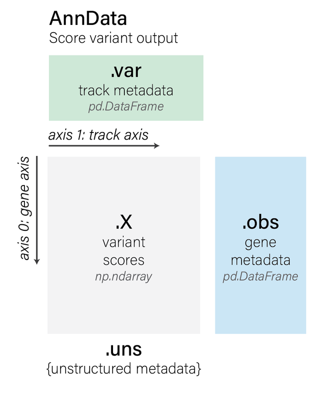
The output of variant scoring is in anndata.AnnData format, which is a way of scoring data together with annotation metadata. Originally developed in the single-cell RNA-seq field, anndata.AnnData is useful when you have metadata associated with an array of data.

anndata.AnnData objects have the following properties (using variant_scores as an example anndata.AnnData object):

variant_scores.X contains a numpy.ndarray containing the variant scores per each gene in the region. This matrix has shape (num_genes, num_tracks), where num_tracks is the number of output tracks in your requested OutputType (such as RNA_SEQ, DNASE, etc.). Note that if you did not use a gene-centric scorer, then variant_scores.X will have shape (1, num_tracks), reflecting the fact that the variant has a single global score and not per-gene score.
variant_scores.var contains the track metadata as a pandas.DataFrame. For every track in the scores (num_genes, num_tracks), there will be a row in the track metadata explaining the track (its cell type, strand, etc.).
variant_scores.obs contains the gene metadata as a pandas.DataFrame. Note that the gene metadata is None in the case of non gene-centric variant scorers.
variant_scores.uns contains some additional unstructured metadata that logs the origin of the variant scores, namely:
- The genome.Variant that was scored (variant_scores.uns[‘variant’])
- The genome.Interval containing the interval (variant_scores.uns[‘interval’])
- The variant scorer that was used to generate the scores (variant_scores.uns[‘scorer’])

From scratch#

You are unlikely to need to create an anndata.AnnData object from scratch, but just for reference, here is how it would be done:

import anndata
import numpy as np
import pandas as pd

# Creating a small matrix of variant scores (3 genes x 2 tracks).
scores = np.array([[0.1, 0.2], [0.3, 0.4], [0.5, 0.6]])

gene_metadata = pd.DataFrame({'gene_id': ['ENSG0001', 'ENSG0002', 'ENSG0003']})

track_metadata = pd.DataFrame(
    {'name': ['track1', 'track2'], 'strand': ['+', '-']}
)

variant_scores = anndata.AnnData(
    X=scores, obs=gene_metadata, var=track_metadata
)

Methods: making predictions#

The main commands for making model predictions are:

dna_client.DnaClient.predict_sequence to predict from a raw DNA string
dna_client.DnaClient.predict_interval to predict from a genome interval (a genome.Interval)
dna_client.DnaClient.predict_variant to make predictions for ref and alt sequences of a variant (a genome.Variant object)
dna_client.DnaClient.score_variant to score the effects of a variant by comparing ref and alt predictions.
dna_client.DnaClient.score_variants the same as the above, but for scoring a list of multiple variants.

Methods: visualization#

The main command for visualizing model predictions is:

alphagenome.visualization.plot_components.plot, to turn a list of of plot components into a matplotlib.figure.Figure.

See the visualization basics guide and visualizing predictions tutorial for more details.

Essential commands

Contents

Essential commands#

Imports#

Data: model inputs#

Genomic interval#

Interval properties#

Resize#

Compare intervals#

Genomic variant#

Insertions or deletions (indels)#

Reference interval#

Overlap with interval#

Data: model outputs#

Track data#

From scratch#

Resolution#

Converting between resolutions#

Filtering#

Resizing#

Slicing#

Subsetting tracks#

Variant scoring output#

#

From scratch#

Methods: making predictions#

Methods: visualization#