Deriving PSI3/5 values from splicing scores

This notebook demonstrates how to derive Percentage Spliced In (PSI) values from predicted splice junction counts.

PSI_5 typically refers to the usage of a 5’ splice site (donor) relative to alternative donors, while PSI_3 refers to the usage of a 3’ splice site (acceptor).

Imports

# @markdown Run this cell to install AlphaGenome.
from IPython.display import clear_output

! pip install alphagenome
clear_output()

from alphagenome import colab_utils
from alphagenome.data import gene_annotation
from alphagenome.data import genome
from alphagenome.data import transcript as transcript_utils
from alphagenome.models import dna_client
from alphagenome.models import variant_scorers
from alphagenome.visualization import plot_components
import matplotlib.pyplot as plt
import pandas as pd

Load the model

dna_model = dna_client.create(colab_utils.get_api_key())

Score a variant

Score a variant near a known splice site:

# Define a variant near a splice site in the BRCA2 gene.
variant = genome.Variant(
    chromosome='chr22',
    position=36201698,
    reference_bases='A',
    alternate_bases='C',
)

# Create a 1MB interval centered on the variant.
interval = variant.reference_interval.resize(dna_client.SEQUENCE_LENGTH_1MB)

# Predict junction counts for both REF and ALT alleles
output = dna_model.predict_variant(
    interval=interval,
    variant=variant,
    requested_outputs=[dna_client.OutputType.SPLICE_JUNCTIONS],
    ontology_terms=['CL:0000084'],
)

There are 107 unique junctions predicted across 2 tracks in this tissue:

print(f"Junctions shape: {output.reference.splice_junctions.junctions.shape}")
print(f"Value shape: {output.reference.splice_junctions.values.shape}")

Junctions shape: (107,)
Value shape: (107, 2)

There are two tracks because splice junction counts are predicted from RNA-seq data, and there are two types of RNA-seq data available for ‘CL:0000084’:

• polyA RNA-seq for mature mRNA splicing because it enriches for fully processed transcripts.

• Total RNA-seq captures pre-mRNA and nascent transcripts, which can sometimes look “messier” because splicing is still in progress.

output.reference.splice_junctions.metadata

	name	ontology_curie	biosample_name	biosample_type	biosample_life_stage	gtex_tissue	data_source	Assay title
0	junction_CL:0000084 polyA plus RNA-seq	CL:0000084	T-cell	primary_cell	adult		encode	polyA plus RNA-seq
1	junction_CL:0000084 total RNA-seq	CL:0000084	T-cell	primary_cell	adult		encode	total RNA-seq

Derive the PSI values

Create a function to calculate PSI values from splice junction counts for either RNA track:

def compute_psi_from_raw(junction_data, track_idx):
  # Create the dataframe from known attributes
  data = []
  for i, j in enumerate(junction_data.junctions):
    # Determine Donor and Acceptor based on strand
    if j.strand == '+':
      donor, acceptor = j.start, j.end
    else:
      donor, acceptor = j.end, j.start

    data.append({
        'donor': donor,
        'acceptor': acceptor,
        'count': junction_data.values[i, track_idx],
    })

  df = pd.DataFrame(data)

  # Pivot into the matrix: Rows = Donors, Cols = Acceptors
  matrix = df.pivot_table(
      index='donor', columns='acceptor', values='count', fill_value=0
  )

  # PSI5: Normalize row-wise (Percent of donor usage for each acceptor)
  # PSI5 = Count / (Total counts for that Donor)
  psi5 = matrix.div(matrix.sum(axis=1), axis=0).fillna(0)

  # PSI3: Normalize column-wise (Percent of acceptor usage for each donor)
  # PSI3 = Count / (Total counts for that Acceptor)
  psi3 = matrix.div(matrix.sum(axis=0), axis=1).fillna(0)

  return psi5, psi3

Select RNA track and calculate:

# We can use either RNA track for PSI values
titles = (
    output.reference.splice_junctions.metadata['Assay title']
    .astype(str)
    .tolist()
)
polya_idx = next(
    (i for i, t in enumerate(titles) if 'polya' in t.lower()), None
)
total_idx = next(
    (i for i, t in enumerate(titles) if 'total' in t.lower()), None
)

# Indecies
print(f'Indices found -> PolyA: {polya_idx}, Total: {total_idx}')

# Calululate PSI
psi5_total, psi3_total = compute_psi_from_raw(
    output.reference.splice_junctions, polya_idx
)

Inspect results

print(
    'The proportion of total splicing activity at a specific acceptor site that'
    ' is contributed by a given donor'
)
display(psi3_total.head())

print(
    'The proportion of total splicing activity at a specific donor site that is'
    ' directed to a given acceptor'
)
display(psi5_total.head())

The proportion of total splicing activity at a specific acceptor site that is contributed by a given donor
The proportion of total splicing activity at a specific donor site that is directed to a given acceptor

acceptor	36191912	36195432	36195437	36197831	36198896	36199369	36199376	36199608	36200291	36201796	36201851	36201888	36202055	36202094	36202933
donor
36192925	0.018779	0.000000	0.000000	0.000000	0.0	0.0	0.0	0.0	0.0	0.0	0.0	0.0	0.0	0.0	0.0
36195094	0.016944	0.000000	0.000000	0.000000	0.0	0.0	0.0	0.0	0.0	0.0	0.0	0.0	0.0	0.0	0.0
36195310	0.908919	0.000000	0.000000	0.000000	0.0	0.0	0.0	0.0	0.0	0.0	0.0	0.0	0.0	0.0	0.0
36195912	0.004811	0.093950	0.016829	0.000000	0.0	0.0	0.0	0.0	0.0	0.0	0.0	0.0	0.0	0.0	0.0
36197944	0.005078	0.087348	0.017657	0.100797	0.0	0.0	0.0	0.0	0.0	0.0	0.0	0.0	0.0	0.0	0.0

acceptor	36191912	36195432	36195437	36197831	36198896	36199369	36199376	36199608	36200291	36201796	36201851	36201888	36202055	36202094	36202933
donor
36192925	1.000000	0.000000	0.000000	0.000000	0.0	0.0	0.0	0.0	0.0	0.0	0.0	0.0	0.0	0.0	0.0
36195094	1.000000	0.000000	0.000000	0.000000	0.0	0.0	0.0	0.0	0.0	0.0	0.0	0.0	0.0	0.0	0.0
36195310	1.000000	0.000000	0.000000	0.000000	0.0	0.0	0.0	0.0	0.0	0.0	0.0	0.0	0.0	0.0	0.0
36195912	0.153461	0.215491	0.631047	0.000000	0.0	0.0	0.0	0.0	0.0	0.0	0.0	0.0	0.0	0.0	0.0
36197944	0.129979	0.160791	0.531372	0.177858	0.0	0.0	0.0	0.0	0.0	0.0	0.0	0.0	0.0	0.0	0.0

Visualise Sashimi plot

As we are considering splicing, we may want to plot more than just protein coding and MANE transcripts. Choose a relevant extractor, but be aware that including all possible transcripts can result in a crowded annotation:

# The GTF file contains information on the location of all transcripts.
# Note that we use genome assembly hg38 for human.
gtf = pd.read_feather(
    'https://storage.googleapis.com/alphagenome/reference/gencode/'
    'hg38/gencode.v46.annotation.gtf.gz.feather'
)

# All transcripts
transcript_extractor_all = transcript_utils.TranscriptExtractor(gtf)

# All protein-coding transcripts
gtf_protein = gene_annotation.filter_protein_coding(gtf)
transcript_extractor_protein = transcript_utils.TranscriptExtractor(gtf_protein)

# All MANE transcripts
gtf_mane = gene_annotation.filter_to_mane_select_transcript(gtf)
transcript_extractor_mane = transcript_utils.TranscriptExtractor(gtf_mane)

# All MANE protein-coding transcripts
gtf_mane_protein = gene_annotation.filter_protein_coding(gtf)
gtf_mane_protein = gene_annotation.filter_to_mane_select_transcript(
    gtf_mane_protein
)
transcript_extractor_mane_protein = transcript_utils.TranscriptExtractor(
    gtf_mane_protein
)

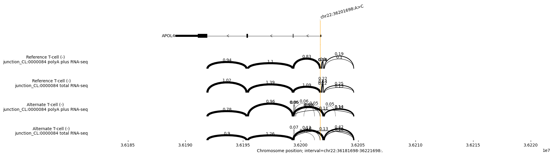
Build the Sashimi plot. The numbers above the junctions in the Sashimi plot are the predicted normalised read counts per donor/acceptor pair (quantitative signal strength). These are NOT the PSI values (proportions):

# We will plot for both polyA and total RNA-seq
ref_output = output.reference
alt_output = output.alternate

# Plot
_ = plot_components.plot(
    [
        # Transcript annotations
        plot_components.TranscriptAnnotation(
            transcript_extractor_mane.extract(interval)
        ),
        # Sashimi ref and alt plots
        plot_components.Sashimi(
            ref_output.splice_junctions,
            ylabel_template='Reference {biosample_name} ({strand})\n{name}',
            color='skyblue',
        ),
        plot_components.Sashimi(
            alt_output.splice_junctions,
            ylabel_template='Alternate {biosample_name} ({strand})\n{name}',
            color='red',
        ),
    ],
    # Annotate the variant position as a vertical line across all panels
    annotations=[plot_components.VariantAnnotation([variant])],
    interval=interval.resize(40000),
)

plt.show()