Key objects

Key objects#

Key activities:

See what dna_model can do, and which output types and conditions it supports
Create and query genome.Interval and genome.Variant objects
Generate and query track_data.TrackData, gene_expression_data.GeneExpressionData, anndata.AnnData, and dna_output.InputGradientsOutput objects

Set up#

# @title Install AlphaGenome

# @markdown Run this cell to install AlphaGenome.
from IPython.display import clear_output
! pip install alphagenome anndata
clear_output()

# @title Imports
from alphagenome import colab_utils
from alphagenome.data import gene_annotation
from alphagenome.data import gene_expression_data
from alphagenome.data import genome
from alphagenome.data import track_data
from alphagenome.models.v2 import dna_client
from alphagenome.models.v2 import variant_scorers
import numpy as np
import pandas as pd

Store your API key in Colab Secrets for persistent access across sessions (see Installation).

dna_model = dna_client.create(colab_utils.get_api_key())

dna_client and dna_model#

dna_client is the module you import. It provides dna_client.create, which connects to the AlphaGenome API with your API key, and the constants used to build requests. The setup cell above calls dna_client.create, which returns a dna_client.DnaClient that we store as dna_model. Every request to the model goes through dna_model:

Task	Method	Returns
Predict tracks for a DNA string, a genome interval, or both alleles of a variant	`dna_model.predict_sequence`, `dna_model.predict_interval`, `dna_model.predict_variant`	`dna_output.Output` (a `dna_output.VariantOutput` with `.reference` and `.alternate` for variants), holding one TrackData per requested output type, or GeneExpressionData for single-cell gene expression
Score a variant or an interval	`dna_model.score_variant`, `dna_model.score_interval`	A list of AnnData objects, one per scorer
Score every single-base substitution in a window (in silico mutagenesis)	`dna_model.score_ism_variants`	A list of AnnData lists, one per variant
List reference conditions and observed training tracks	`dna_model.supported_conditions`, `dna_model.observed_metadata`	A pandas DataFrame; a `dna_output.OutputMetadata`
Embed your own cells for expression conditioning	`dna_model.encode_cells`	A NumPy array with one embedding per cell
Compute input gradients of a gene’s predicted expression	`dna_model.predict_interval_gradients`	A `dna_output.InputGradientsOutput`

The batch methods dna_model.predict_sequences, dna_model.predict_intervals, dna_model.predict_variants, dna_model.score_intervals, dna_model.score_variants, and dna_model.predict_interval_gradients_batch take lists (with one reference condition via conditions= or expression-conditioning input via cell_conditionings= plus cell_condition_names= per item) and return one result per item. The sections below cover each return type: TrackData, GeneExpressionData, AnnData, and InputGradientsOutput.

dna_client also defines the constants used in requests: dna_client.OutputType (what to predict), dna_client.Organism (human or mouse), the supported input lengths (dna_client.SEQUENCE_LENGTH_16KB to dna_client.SEQUENCE_LENGTH_1MB; input gradients support SEQUENCE_LENGTH_100KB and SEQUENCE_LENGTH_1MB), dna_client.MAX_CONDITIONING_CELLS (256 cells per expression conditioning call), and dna_client.ModelVersion.

Output types#

The model can make predictions for the following output types:

# Observe available output types in dna_client.
[output.name for output in dna_client.OutputType]

['ATAC',
 'CAGE',
 'DNASE',
 'RNA_SEQ',
 'CHIP_HISTONE',
 'CHIP_TF',
 'SPLICE_SITES',
 'SPLICE_SITE_USAGE',
 'SPLICE_JUNCTIONS',
 'CONTACT_MAPS',
 'SC_GENE_EXPRESSION',
 'SC_ATAC',
 'SC_GENE_EXPRESSION_DENOISED',
 'CELL_EMBEDDINGS',
 'METHYLATION']

Supported OutputType values span bulk genomic assays, single-cell expression and chromatin accessibility (denoised SC_GENE_EXPRESSION_DENOISED under cell_conditioning=, plus protocol-specific SC_GENE_EXPRESSION and SC_ATAC), splicing readouts, 3D contact maps, and base-resolution CpG methylation. See Model output metadata for units, resolution, and track counts per output type.

Conditions#

AlphaGenome 2 supports two workflows for conditioning predictions on cellular context:

Reference conditions: pass a reference ontology CURIE or model_condition.ModelCondition via condition= (retrievable with dna_client.DnaClient.supported_conditions).
Expression conditioning: pass your own human scRNA-seq counts via cell_conditioning= alongside cell_condition_name=; see Conditioning on your own single-cell data.

Composite conditions join ontology CURIEs from CLO, UBERON, CL, EFO, and NTR with _, typically pairing a tissue UBERON CURIE with a cell-type CL CURIE such as UBERON:0000178_CL:0001054 (CD14-positive monocytes in blood) or UBERON:0009834_CL:0000129 (frontal cortex microglia), while most bulk conditions use a single CURIE.

dna_model.supported_conditions returns a pandas.DataFrame where each row is one reference condition, with columns condition, biosample_type, biosample_name, and one imputation-mode column per output type:

# Explore available conditions in dna_client.
supported_conditions = dna_model.supported_conditions(
    dna_client.Organism.HOMO_SAPIENS
)
supported_conditions.head(10)

	condition	biosample_type	biosample_name	atac	cage	dnase	rna_seq	chip_histone	chip_tf	splice_sites	splice_site_usage	splice_junctions	contact_maps	sc_atac	sc_gene_expression	methylation
0	CL:0000047	primary_cell	neural stem cell	imputed_supported	imputed_exploratory	observed	observed	observed	imputed_exploratory	observed	observed	observed	imputed_exploratory	imputed_supported	imputed_supported	imputed_supported
1	CL:0000100	in_vitro_differentiated_cells	motor neuron	observed	imputed_exploratory	imputed_supported	observed	observed	imputed_exploratory	observed	observed	observed	imputed_exploratory	imputed_supported	imputed_supported	imputed_supported
2	CL:0000115	primary_cell	endothelial cell	imputed_supported	imputed_exploratory	observed	observed	imputed_supported	observed	imputed_exploratory	imputed_exploratory	imputed_exploratory	imputed_exploratory	imputed_supported	imputed_supported	imputed_supported
3	CL:0000134	primary_cell	mesenchymal stem cell	imputed_supported	imputed_exploratory	observed	observed	observed	imputed_exploratory	observed	observed	observed	imputed_exploratory	imputed_supported	imputed_supported	imputed_supported
4	CL:0000136	primary_cell	adipocyte	imputed_supported	imputed_exploratory	observed	imputed_supported	observed	imputed_exploratory	imputed_exploratory	imputed_exploratory	imputed_exploratory	imputed_exploratory	imputed_supported	imputed_supported	imputed_supported
5	CL:0000137	primary_cell	osteocyte	imputed_supported	imputed_exploratory	observed	observed	imputed_supported	observed	imputed_exploratory	imputed_exploratory	imputed_exploratory	imputed_exploratory	imputed_supported	imputed_supported	imputed_supported
6	CL:0000138	primary_cell	chondrocyte	imputed_supported	imputed_exploratory	observed	observed	imputed_supported	observed	imputed_exploratory	imputed_exploratory	imputed_exploratory	imputed_exploratory	imputed_supported	imputed_supported	imputed_supported
7	CL:0000169	primary_cell	type B pancreatic cell	imputed_supported	imputed_exploratory	observed	observed	imputed_supported	observed	imputed_exploratory	imputed_exploratory	imputed_exploratory	imputed_exploratory	imputed_supported	imputed_supported	imputed_supported
8	CL:0000182	primary_cell	hepatocyte	imputed_supported	imputed_exploratory	observed	observed	observed	observed	observed	observed	observed	imputed_exploratory	imputed_supported	imputed_supported	imputed_supported
9	CL:0000187	primary_cell	muscle cell	imputed_supported	imputed_exploratory	observed	observed	imputed_supported	imputed_exploratory	observed	observed	observed	imputed_exploratory	imputed_supported	imputed_supported	imputed_supported

Every supported condition predicts all output types, labeling each track as observed, imputed_supported, or imputed_exploratory in metadata['imputation_mode']. See Navigating imputed tracks for guidance on each mode.

Filtering the table shows, for example, that microglia have separate composite conditions for frontal cortex (UBERON:0009834_CL:0000129) and macula lutea in the retina (UBERON:0000053_CL:0000129):

dna_model.supported_conditions().query(
    'condition == ["UBERON:0009834_CL:0000129",'
    ' "UBERON:0000053_CL:0000129"]'
)

	condition	biosample_type	biosample_name	atac	cage	dnase	rna_seq	chip_histone	chip_tf	splice_sites	splice_site_usage	splice_junctions	contact_maps	sc_atac	sc_gene_expression	methylation
351	UBERON:0000053_CL:0000129	primary_cell	macula lutea microglial cell	imputed_supported	imputed_exploratory	imputed_supported	imputed_supported	imputed_supported	imputed_exploratory	imputed_exploratory	imputed_exploratory	imputed_exploratory	imputed_exploratory	observed	observed	imputed_supported
2649	UBERON:0009834_CL:0000129	primary_cell	dorsolateral prefrontal cortex microglial cell	imputed_supported	imputed_exploratory	imputed_supported	imputed_supported	imputed_supported	imputed_exploratory	imputed_exploratory	imputed_exploratory	imputed_exploratory	imputed_exploratory	observed	observed	imputed_supported

genome.Interval#

A genome.Interval object is used to define a continuous genomic coordinate window. Intervals in AlphaGenome use a 0-based coordinate system. An interval can be set directly using coordinates, from a string, or by fetching gene coordinates from the GTF annotation file.

Intervals use half-open [start, end) coordinates on human (hg38) or mouse (mm10) assemblies.

Create#

# Define interval directly...
interval = genome.Interval(
    chromosome='chr22',
    start=36_189_123,
    end=36_204_840,
    strand='-',  # Default is unstranded (.).
)

# Or by parsing a string...
interval = genome.Interval.from_str('chr22:36189123-36204840')

# Or by fetching an interval around a gene using either HGNC or ENSEMBL gene_id.
gtf = pd.read_feather(
    'https://storage.googleapis.com/alphagenome/reference/gencode/'
    'hg38/gencode.v46.annotation.gtf.gz.feather'
)
interval = gene_annotation.get_gene_interval(gtf, gene_symbol='APOL4')

Resize#

The .resize() method adjusts the interval to the specified width by expanding (or contracting) around its original center, incorporating more bases from the reference genomic sequence rather than padding tokens. This method can be used to resize the interval to a model-compatible length.

# Resizing the interval into the center.
smaller_interval = interval.resize(100)

# Resizing the interval around the center to make compatible with model.
resized_interval = interval.resize(dna_client.SEQUENCE_LENGTH_1MB)

Important

Use a 1 Mb interval (dna_client.SEQUENCE_LENGTH_1MB) for best accuracy. See Selecting a genomic region for all supported lengths.

In order to make interval or variant predictions the interval must be of a model-compatible size

# Model-compatible interval sequence lengths.
list(dna_client.SUPPORTED_SEQUENCE_LENGTHS.keys())

['SEQUENCE_LENGTH_16KB',
 'SEQUENCE_LENGTH_100KB',
 'SEQUENCE_LENGTH_500KB',
 'SEQUENCE_LENGTH_1MB']

Properties#

After resizing to 1 Mb, the interval width is 1,048,576 bp (\(2^{20}\)), matching dna_client.SEQUENCE_LENGTH_1MB:

# Fetch interval width.
print(f"Interval width: {interval.width}\n")
print(f"Resized interval width: {resized_interval.width}")

Interval width: 15717

Resized interval width: 1048576

# Fetch centre of an interval.
interval.center()

36196981

Compare intervals#

print(f"Intervals overlap?: {interval.overlaps(resized_interval)}")
print(
    "Interval contains resized interval?:"
    f" {interval.contains(resized_interval)}"
)
print(
    "What is the intersection of the intervals?:"
    f" {interval.intersect(resized_interval)}"
)

Intervals overlap?: True
Interval contains resized interval?: False
What is the intersection of the intervals?: chr22:36189123-36204840:-

genome.Variant#

A genome.Variant object is used to define a variant. Variants in AlphaGenome use a 1-based coordinate system. Variants can be single base variants (SNVs) or indels.

Both reference_bases and alternate_bases use uppercase base characters (A, C, G, T).

Create an SNV#

# SNV variant.
variant = genome.Variant(
    chromosome='chr3', position=10_000, reference_bases='A', alternate_bases='C'
)

print(f'Variant: {variant}')

Variant: chr3:10000:A>C

Create an indel#

# Insertion variant.
variant_in = genome.Variant(
    chromosome='chr3',
    position=10_000,
    reference_bases='T',
    alternate_bases='CGTCAAT',
)

# Deletion variant.
variant_del = genome.Variant(
    chromosome='chr3',
    position=10_000,
    reference_bases='AGGGATC',
    alternate_bases='C',
)

The sequence we pass for the reference_bases argument can differ from what is actually at that location in the hg38/mm10 reference genome. The model will insert whatever is passed as the reference and alternate bases into the sequence and make predictions on them.

Reference interval#

We can get the genome.Interval corresponding to the reference bases of the variant

variant.reference_interval

Interval(chromosome='chr3', start=9999, end=10000, strand='.', name='')

A common use-case is to make predictions in a genome region around a variant, which involves resizing the genome.Variant.reference_interval to a sequence length compatible with AlphaGenome:

# Fetch 1 Mb reference interval around the variant.
variant_interval = variant.reference_interval.resize(
    dna_client.SEQUENCE_LENGTH_1MB
)
variant_interval.width

Overlap with interval#

We can also check if a variant’s reference or alternate alleles overlap a genome.Interval

variant = genome.Variant(
    chromosome='chr3',
    position=10_000,
    reference_bases='T',
    alternate_bases='CGTCAAT',
)

interval = genome.Interval(chromosome='chr3', start=10_005, end=10_010)

print('Reference overlaps:', variant.reference_overlaps(interval))
print('Alternative overlaps:', variant.alternate_overlaps(interval))

Reference overlaps: False
Alternative overlaps: True

TrackData (track predictions)#

When we make track predictions, the results are stored in a track_data.TrackData object.

Generating TrackData from predictions#

Here we predict DNase-seq (dna_client.OutputType.DNASE) for lung (UBERON:0002048):

output = dna_model.predict_sequence(
    sequence='GATTACA'.center(dna_client.SEQUENCE_LENGTH_16KB, 'N'),  # Pad to valid sequence length.
    requested_outputs=[dna_client.OutputType.DNASE],
    condition='UBERON:0002048',  # Lung.
)

The output object contains predictions for all the different requested output types (in this case, only output type DNASE). Predictions for genomic tracks are stored inside a TrackData object

dnase_tdata = output.dnase
type(dnase_tdata)

alphagenome.data.track_data.TrackData

TrackData objects have the following components:

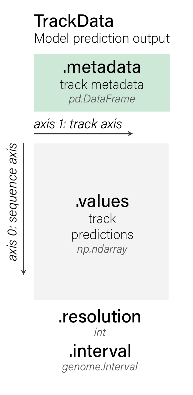
track_data.TrackData objects store model predictions. They have the following properties (using tdata as an example of a track_data.TrackData object):

tdata.values store track predictions as a numpy.ndarray .
tdata.metadata stores track metadata as a pandas.DataFrame. For each track in the predicted values, there will be a corresponding row in the track metadata describing its origin.
tdata.uns contains additional unstructured metadata as a dict.

The predictions of shape (sequence_length, num_tracks) are stored in .values:

print(dnase_tdata.values.shape)

dnase_tdata.values

(16384, 2)

array([[8.0588696e-05, 1.4885553e-04],
       [1.1215313e-05, 1.7122606e-05],
       [2.0550968e-05, 2.8056431e-05],
       ...,
       [7.0503855e-05, 5.9202735e-05],
       [1.4437331e-04, 1.1177733e-04],
       [2.1921449e-04, 2.2257322e-04]], shape=(16384, 2), dtype=float32)

And the corresponding metadata describing each of the tracks is stored in .metadata:

dnase_tdata.metadata

	name	strand	biosample_curie	imputation_mode	biosample_type	biosample_name	Assay title	data_source	genetically_modified	endedness	data_pipeline
0	UBERON:0002048_DNase-seq-encode-paired-ended	.	UBERON:0002048	observed	tissue	lung	DNase-seq	encode	False	paired	encode
1	UBERON:0002048_DNase-seq-encode-single-ended	.	UBERON:0002048	observed	tissue	lung	DNase-seq	encode	False	single	encode

The .metadata DataFrame has one row per returned track, matching the second dimension of .values.

The track metadata is especially useful when requesting predictions for stranded assays (which have separate readouts for the two DNA strands, such as CAGE and RNA_SEQ), and for checking whether each track is observed or imputed.

output = dna_model.predict_sequence(
    sequence='GATTACA'.center(dna_client.SEQUENCE_LENGTH_16KB, 'N'),  # Pad to valid sequence length.
    requested_outputs=[
        dna_client.OutputType.CAGE,
        dna_client.OutputType.DNASE,
    ],
    condition='UBERON:0000955',  # Brain.
)

print(f'DNASE predictions shape: {output.dnase.values.shape}')
print(f'CAGE predictions shape: {output.cage.values.shape}')

DNASE predictions shape: (16384, 2)
CAGE predictions shape: (16384, 4)

Notice that in this example, we requested predictions for 2 output types simultaneously.

The CAGE track metadata describes the strand and assay source of each predicted track:

output.cage.metadata

	name	strand	biosample_curie	imputation_mode	biosample_type	biosample_name	Assay title	data_pipeline	data_source
0	UBERON:0000955_LQhCAGE-fantom	+	UBERON:0000955	imputed_exploratory	tissue	brain	LQhCAGE	fantom	NaN
1	UBERON:0000955_hCAGE-fantom	+	UBERON:0000955	observed	tissue	brain	hCAGE	fantom	fantom
2	UBERON:0000955_LQhCAGE-fantom	-	UBERON:0000955	imputed_exploratory	tissue	brain	LQhCAGE	fantom	NaN
3	UBERON:0000955_hCAGE-fantom	-	UBERON:0000955	observed	tissue	brain	hCAGE	fantom	fantom

We can easily filter the TrackData object for only observed tracks.

# : indexes the positional axis while the boolean mask indexes into tracks.
observed_mask = (output.cage.metadata.imputation_mode == 'observed').values
subset_cage = output.cage[:, observed_mask]
subset_cage.metadata

	name	strand	biosample_curie	imputation_mode	biosample_type	biosample_name	Assay title	data_pipeline	data_source
1	UBERON:0000955_hCAGE-fantom	+	UBERON:0000955	observed	tissue	brain	hCAGE	fantom	fantom
3	UBERON:0000955_hCAGE-fantom	-	UBERON:0000955	observed	tissue	brain	hCAGE	fantom	fantom

Creating TrackData from scratch#

You can create your own track_data.TrackData object from scratch by specifying the values and metadata manually. The metadata must contain at least the columns name (the names of the tracks) and strand (the strands of DNA that the tracks are on):

# Array has shape (4,3) -> sequence is length 4 and there are 3 tracks.
values = np.array([[0, 1, 2], [3, 4, 5], [6, 7, 8], [9, 10, 11]]).astype(
    np.float32
)

# We have both the positive and negative strand values for track1, while track2.
# Contains unstranded data.
metadata = pd.DataFrame({
    'name': ['track1', 'track1', 'track2'],
    'strand': ['+', '-', '.'],
})

tdata = track_data.TrackData(values=values, metadata=metadata)

It’s also useful to specify the resolution of the tracks and the genomic interval that they come from, if you have this information available

interval = genome.Interval(chromosome='chr1', start=1_000, end=1_004)
tdata = track_data.TrackData(
    values=values, metadata=metadata, resolution=1, interval=interval
)

Note that the length of the values has to match up with the interval width and resolution. Here is an example specifying that the values actually represent 128 bp resolution tracks (i.e., each number is a summary over 128 base pairs of DNA):

interval = genome.Interval(chromosome='chr1', start=1_000, end=1_512)
tdata = track_data.TrackData(
    values=values, metadata=metadata, resolution=128, interval=interval
)

We can also interconvert between resolutions. For example, given 1 bp resolution predictions, we can downsample the resolution (by summing adjacent values) and return a sequence of length 2:

interval = genome.Interval(chromosome='chr1', start=1_000, end=1_004)

tdata = track_data.TrackData(
    values=values, metadata=metadata, resolution=1, interval=interval
)

tdata = tdata.change_resolution(resolution=2)
tdata.values

array([[ 3.,  5.,  7.],
       [15., 17., 19.]], dtype=float32)

We can also upsample track data to get back to 1 bp resolution and a sequence of length 4 by repeating values while preserving the sum:

tdata = tdata.change_resolution(resolution=1)
tdata.values

array([[1.5, 2.5, 3.5],
       [1.5, 2.5, 3.5],
       [7.5, 8.5, 9.5],
       [7.5, 8.5, 9.5]], dtype=float32)

Filtering#

track_data.TrackData objects can be filtered by the type of DNA strand the tracks are on.

print(
    'Positive strand tracks:',
    tdata.filter_to_positive_strand().metadata.name.values,
)
print(
    'Negative strand tracks:',
    tdata.filter_to_negative_strand().metadata.name.values,
)
print('Unstranded tracks:', tdata.filter_to_unstranded().metadata.name.values)

Positive strand tracks: ['track1']
Negative strand tracks: ['track1']
Unstranded tracks: ['track2']

Resizing#

We can resize the track_data.TrackData to be either smaller (by cropping)

# Re-instantiating the original trackdata.
tdata = track_data.TrackData(
    values=values, metadata=metadata, resolution=1, interval=interval
)

# Resize from width (sequence length) of 4 down to 2.
tdata.resize(width=2).values

array([[3., 4., 5.],
       [6., 7., 8.]], dtype=float32)

Or bigger (by padding with zeros):

tdata.resize(width=8).values

array([[ 0.,  0.,  0.],
       [ 0.,  0.,  0.],
       [ 0.,  1.,  2.],
       [ 3.,  4.,  5.],
       [ 6.,  7.,  8.],
       [ 9., 10., 11.],
       [ 0.,  0.,  0.],
       [ 0.,  0.,  0.]], dtype=float32)

Slicing#

We can slice into specific positions of the track_data.TrackData:

# Get the final 2 positions only.
print('slice by position: ', tdata.slice_by_positions(start=2, end=4).values)
# Same, but using slice_interval:
print(
    'slice by interval: ',
    tdata.slice_by_interval(
        genome.Interval(chromosome='chr1', start=1_002, end=1_004)
    ).values,
)

slice by position:  [[ 6.  7.  8.]
 [ 9. 10. 11.]]
slice by interval:  [[ 6.  7.  8.]
 [ 9. 10. 11.]]

Subsetting#

Subset (and reorder) to specific track names

# Get only tracks with the name 'track1'.
track1_tdata = tdata.select_tracks_by_name(names='track1')
track1_tdata.values

array([[ 0.,  1.],
       [ 3.,  4.],
       [ 6.,  7.],
       [ 9., 10.]], dtype=float32)

The metadata gets automatically filtered to track1 too:

track1_tdata.metadata.name.values

array(['track1', 'track1'], dtype=object)

Slicing and filtering with `[]` access.#

We can also apply operations using [] notation like numpy arrays, which generalizes the methods applied above to position and track axes.

interval_and_track_sliced = tdata[
    genome.Interval(chromosome='chr1', start=1_002, end=1_004),
    (tdata.metadata.name == 'track1').values,
]
print(
    'slice by interval and boolean track mask: ',
    interval_and_track_sliced.values,
)

position_and_track_sliced = tdata[2:4, 0:2]
print('slice using python slices: ', position_and_track_sliced.values)

position_and_track_sliced = tdata[2:4, ['track1']]
print('slice using slices and track names: ', position_and_track_sliced.values)

slice by interval and boolean track mask:  [[ 6.  7.]
 [ 9. 10.]]
slice using python slices:  [[ 6.  7.]
 [ 9. 10.]]
slice using slices and track names:  [[ 6.  7.]
 [ 9. 10.]]

Finally, if we pass in a stranded genome.Interval or leave unspecified as None when constructing a track_data.TrackData, we can reverse complement transform our track values in a strand-aware manner:

interval = genome.Interval(
    chromosome='chr1', start=1_000, end=1_004, strand='+'
)

tdata = track_data.TrackData(
    values=values, metadata=metadata, resolution=1, interval=interval
)

tdata.reverse_complement().values

array([[10.,  9., 11.],
       [ 7.,  6.,  8.],
       [ 4.,  3.,  5.],
       [ 1.,  0.,  2.]], dtype=float32)

To plot TrackData, wrap it in plot components and render them with plot_components.plot; see Plotting predictions.

GeneExpressionData (gene expression predictions)#

Gene-level single-cell expression predictions (SC_GENE_EXPRESSION_DENOISED for denoised single-cell gene expression under cell_conditioning=, and SC_GENE_EXPRESSION for protocol-specific channels across reference and expression conditioning) are stored in a gene_expression_data.GeneExpressionData object rather than a TrackData object, indexed by annotated genes ((num_genes, num_tracks), in CPM) rather than base-pair positions.

Creating GeneExpressionData from scratch#

Just like TrackData, we can inspect the structure of gene_expression_data.GeneExpressionData by instantiating one directly from a (num_genes, num_tracks) array, a gene_metadata DataFrame, a track_metadata DataFrame, and a genome.Interval:

interval = genome.Interval(chromosome='chr22', start=36_150_000, end=36_270_000)
values = np.array([[12.5, 0.2], [0.1, 8.4], [3.1, 0.0]], dtype=np.float32)
gene_metadata = pd.DataFrame({
    'gene_id': ['ENSG00000100342', 'ENSG00000100345', 'ENSG00000273079'],
    'gene_name': ['APOL1', 'MYH9', 'APOL1-AS1'],
    'gene_type': ['protein_coding', 'protein_coding', 'lncRNA'],
    'Chromosome': ['chr22', 'chr22', 'chr22'],
    'Start': [36_253_071, 36_162_688, 36_245_000],
    'End': [36_267_531, 36_230_000, 36_252_000],
    'strand': ['+', '-', '-'],
})
track_metadata = pd.DataFrame({
    'name': ['scRNA_pos', 'scRNA_neg'],
    'strand': ['+', '-'],
    'imputation_mode': ['observed', 'observed'],
})

gdata = gene_expression_data.GeneExpressionData(
    values=values,
    gene_metadata=gene_metadata,
    track_metadata=track_metadata,
    interval=interval,
)
print(f'Values shape (num_genes, num_tracks): {gdata.values.shape}')
gdata.gene_metadata

Values shape (num_genes, num_tracks): (3, 2)

	gene_id	gene_name	gene_type	Chromosome	Start	End	strand
0	ENSG00000100342	APOL1	protein_coding	chr22	36253071	36267531	+
1	ENSG00000100345	MYH9	protein_coding	chr22	36162688	36230000	-
2	ENSG00000273079	APOL1-AS1	lncRNA	chr22	36245000	36252000	-

Filtering and resizing#

GeneExpressionData provides convenience methods for filtering track columns by strand (such as filter_to_positive_strand), filtering gene rows to protein-coding genes (filter_to_protein_coding), slicing gene rows by metadata mask, and retaining genes that overlap a genomic sub-interval (slice_by_interval / resize):

coding_pos_gdata = gdata.filter_to_protein_coding().filter_to_positive_strand()
coding_pos_gdata = coding_pos_gdata[coding_pos_gdata.gene_metadata['strand'] == '+']
print(
    'Protein-coding + strand genes on + track:',
    coding_pos_gdata.gene_metadata.gene_name.tolist(),
)
print('Filtered shape:', coding_pos_gdata.values.shape)

sliced_gdata = gdata.slice_by_interval(
    genome.Interval(chromosome='chr22', start=36_240_000, end=36_270_000)
)
print(
    'Genes overlapping chr22:36240000-36270000:',
    sliced_gdata.gene_metadata.gene_name.tolist(),
)

Protein-coding + strand genes on + track: ['APOL1']
Filtered shape: (1, 1)
Genes overlapping chr22:36240000-36270000: ['APOL1', 'APOL1-AS1']

Slicing with `[]` and converting to `AnnData`#

We can index GeneExpressionData using [gene_idx, track_idx] (matching Ensembl gene_id values and track name values), or convert directly to an anndata.AnnData object via gene_expression_data.GeneExpressionData.to_anndata:

subset_gdata = gdata[['ENSG00000100342', 'ENSG00000100345'], ['scRNA_pos']]
print('Sliced values:\n', subset_gdata.values)

adata = gdata.to_anndata()
adata

Sliced values:
 [[12.5]
 [ 0.1]]

AnnData object with n_obs × n_vars = 3 × 2
    obs: 'gene_id', 'gene_name', 'gene_type', 'Chromosome', 'Start', 'End', 'strand'
    var: 'name', 'strand', 'imputation_mode'
    uns: 'interval'
    layers: None (.X)

AnnData (variant scoring)#

When we score variants, the results for the specified condition are stored in an anndata.AnnData object.

Generating AnnData from variant scoring#

# Set a variant and interval.
variant = genome.Variant(
    chromosome='chr22',
    position=36201698,
    reference_bases='A',
    alternate_bases='C',
)
interval = variant.reference_interval.resize(dna_client.SEQUENCE_LENGTH_1MB)

# Score a variant using the RNA_SEQ recommended scorer.
variant_scorer = variant_scorers.RECOMMENDED_VARIANT_SCORERS['RNA_SEQ']

variant_scores = dna_model.score_variant(
    interval=interval,
    variant=variant,
    variant_scorers=[variant_scorer],
    condition='UBERON:0002048',  # Lung.
)

AnnData objects have the following components:

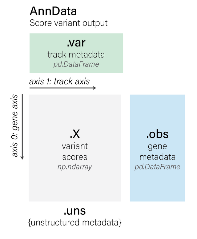
The output of variant scoring is in anndata.AnnData format, which stores a score matrix alongside row and column annotations.

anndata.AnnData objects returned by score_variant have the following properties (using variant_scores as an example):

variant_scores.X contains a numpy.ndarray of variant scores with shape (num_rows, num_tracks), where num_tracks is the number of tracks in the requested OutputType. For gene-centric scorers, rows index annotated genes ((num_genes, num_tracks)); for CenterMaskScorer and ContactMapScorer, shape is (1, num_tracks); for CpG methylation and splice junction scorers, rows index CpG sites or splice junctions.
variant_scores.var contains the track metadata as a pandas.DataFrame (one row per track).
variant_scores.obs contains row metadata as a pandas.DataFrame (gene metadata for gene-centric scorers, CpG or junction metadata where applicable, or empty for single-row CenterMaskScorer outputs).
variant_scores.uns stores unstructured provenance metadata:
- The genome.Variant that was scored (variant_scores.uns['variant'])
- The genome.Interval used as context (variant_scores.uns['interval'])
- The variant scorer configuration (variant_scores.uns['variant_scorer'])

Properties#

The returned variant_scores is a list of length 1 because we only specified 1 scorer:

len(variant_scores)

Unpack the first scorer’s AnnData object:

variant_scores = variant_scores[0]
variant_scores

AnnData object with n_obs × n_vars = 37 × 5
    obs: 'gene_id', 'strand', 'gene_name', 'gene_type'
    var: 'name', 'strand', 'biosample_curie', 'imputation_mode', 'biosample_type', 'biosample_name', 'Assay title', 'data_source', 'genetically_modified', 'endedness', 'data_pipeline'
    uns: 'interval', 'variant', 'variant_scorer'
    layers: None (.X)

The matrix in .X has one row per gene in the interval and one column per RNA_SEQ track:

variant_scores.X.shape

(37, 5)

The description of each track is accessed using .var (this is the same dataframe as the output metadata, but is included alongside the variant scores for convenience):

variant_scores.var.head()

	name	strand	biosample_curie	imputation_mode	biosample_type	biosample_name	Assay title	data_source	genetically_modified	endedness	data_pipeline
0	UBERON:0002048_polyA plus RNA-seq-encode-paire...	.	UBERON:0002048	observed	tissue	lung	polyA plus RNA-seq	encode	False	paired	encode
1	UBERON:0002048_polyA plus RNA-seq-encode-singl...	.	UBERON:0002048	imputed_supported	tissue	lung	polyA plus RNA-seq	NaN	NaN	single	encode
2	UBERON:0002048_total RNA-seq-encode-paired-ended	.	UBERON:0002048	observed	tissue	lung	total RNA-seq	encode	False	paired	encode
3	UBERON:0002048_total RNA-seq-encode-single-ended	.	UBERON:0002048	observed	tissue	lung	total RNA-seq	encode	False	single	encode
4	UBERON:0002048_polyA plus RNA-seq-gtex-paired-...	.	UBERON:0002048	imputed_supported	tissue	lung	polyA plus RNA-seq	NaN	NaN	paired	recount3

We can inspect the gene metadata in .obs. Here are the first 5 genes:

variant_scores.obs.head()

	gene_id	strand	gene_name	gene_type
0	ENSG00000100320.24	-	RBFOX2	protein_coding
1	ENSG00000100336.18	-	APOL4	protein_coding
2	ENSG00000100342.22	+	APOL1	protein_coding
3	ENSG00000100345.23	-	MYH9	protein_coding
4	ENSG00000100348.10	-	TXN2	protein_coding

Some handy additional metadata can be found in .uns:

print(f'Interval: {variant_scores.uns["interval"]}')
print(f'Variant: {variant_scores.uns["variant"]}')
print(f'Variant scorer: {variant_scores.uns["variant_scorer"]}')

Interval: chr22:35677410-36725986:.
Variant: chr22:36201698:A>C
Variant scorer: GeneMaskLFCScorer(requested_output=RNA_SEQ, aggregation_type=DIFF_MEAN)

Spatial scorers without per-feature rows (such as variant_scorers.CenterMaskScorer and variant_scorers.ContactMapScorer) return shape (1, num_tracks), whereas methylation and splice junction scorers index CpG sites or splice junctions along .obs.

Flattening#

We recommend interacting with variant scores by flattening AnnData objects using variant_scorers.tidy_scores. It optionally excludes stranded tracks which do not match the gene’s strand for gene-specific scorer. The raw_score column contains the same values as stored in variant_scores.X.

variant_scorers.tidy_scores([variant_scores], match_gene_strand=True)

	variant_id	scored_interval	gene_id	gene_name	gene_type	gene_strand	junction_Start	junction_End	output_type	variant_scorer	track_name	track_strand	imputation_mode	biosample_curie	biosample_type	biosample_name	Assay title	data_source	genetically_modified	endedness	data_pipeline	raw_score
0	chr22:36201698:A>C	chr22:35677410-36725986:.	ENSG00000100320	RBFOX2	protein_coding	-	None	None	RNA_SEQ	GeneMaskLFCScorer(requested_output=RNA_SEQ, ag...	UBERON:0002048_polyA plus RNA-seq-encode-paire...	.	observed	UBERON:0002048	tissue	lung	polyA plus RNA-seq	encode	False	paired	encode	-0.000960
1	chr22:36201698:A>C	chr22:35677410-36725986:.	ENSG00000100320	RBFOX2	protein_coding	-	None	None	RNA_SEQ	GeneMaskLFCScorer(requested_output=RNA_SEQ, ag...	UBERON:0002048_polyA plus RNA-seq-encode-singl...	.	imputed_supported	UBERON:0002048	tissue	lung	polyA plus RNA-seq	NaN	NaN	single	encode	0.000123
2	chr22:36201698:A>C	chr22:35677410-36725986:.	ENSG00000100320	RBFOX2	protein_coding	-	None	None	RNA_SEQ	GeneMaskLFCScorer(requested_output=RNA_SEQ, ag...	UBERON:0002048_total RNA-seq-encode-paired-ended	.	observed	UBERON:0002048	tissue	lung	total RNA-seq	encode	False	paired	encode	0.001117
3	chr22:36201698:A>C	chr22:35677410-36725986:.	ENSG00000100320	RBFOX2	protein_coding	-	None	None	RNA_SEQ	GeneMaskLFCScorer(requested_output=RNA_SEQ, ag...	UBERON:0002048_total RNA-seq-encode-single-ended	.	observed	UBERON:0002048	tissue	lung	total RNA-seq	encode	False	single	encode	0.000609
4	chr22:36201698:A>C	chr22:35677410-36725986:.	ENSG00000100320	RBFOX2	protein_coding	-	None	None	RNA_SEQ	GeneMaskLFCScorer(requested_output=RNA_SEQ, ag...	UBERON:0002048_polyA plus RNA-seq-gtex-paired-...	.	imputed_supported	UBERON:0002048	tissue	lung	polyA plus RNA-seq	NaN	NaN	paired	recount3	0.000051
...	...	...	...	...	...	...	...	...	...	...	...	...	...	...	...	...	...	...	...	...	...	...
180	chr22:36201698:A>C	chr22:35677410-36725986:.	ENSG00000293594	ENSG00000293594	processed_pseudogene	-	None	None	RNA_SEQ	GeneMaskLFCScorer(requested_output=RNA_SEQ, ag...	UBERON:0002048_polyA plus RNA-seq-encode-paire...	.	observed	UBERON:0002048	tissue	lung	polyA plus RNA-seq	encode	False	paired	encode	0.009897
181	chr22:36201698:A>C	chr22:35677410-36725986:.	ENSG00000293594	ENSG00000293594	processed_pseudogene	-	None	None	RNA_SEQ	GeneMaskLFCScorer(requested_output=RNA_SEQ, ag...	UBERON:0002048_polyA plus RNA-seq-encode-singl...	.	imputed_supported	UBERON:0002048	tissue	lung	polyA plus RNA-seq	NaN	NaN	single	encode	0.004218
182	chr22:36201698:A>C	chr22:35677410-36725986:.	ENSG00000293594	ENSG00000293594	processed_pseudogene	-	None	None	RNA_SEQ	GeneMaskLFCScorer(requested_output=RNA_SEQ, ag...	UBERON:0002048_total RNA-seq-encode-paired-ended	.	observed	UBERON:0002048	tissue	lung	total RNA-seq	encode	False	paired	encode	0.006874
183	chr22:36201698:A>C	chr22:35677410-36725986:.	ENSG00000293594	ENSG00000293594	processed_pseudogene	-	None	None	RNA_SEQ	GeneMaskLFCScorer(requested_output=RNA_SEQ, ag...	UBERON:0002048_total RNA-seq-encode-single-ended	.	observed	UBERON:0002048	tissue	lung	total RNA-seq	encode	False	single	encode	0.005193
184	chr22:36201698:A>C	chr22:35677410-36725986:.	ENSG00000293594	ENSG00000293594	processed_pseudogene	-	None	None	RNA_SEQ	GeneMaskLFCScorer(requested_output=RNA_SEQ, ag...	UBERON:0002048_polyA plus RNA-seq-gtex-paired-...	.	imputed_supported	UBERON:0002048	tissue	lung	polyA plus RNA-seq	NaN	NaN	paired	recount3	0.009735

185 rows × 22 columns

Creating AnnData from scratch#

You are unlikely to need to create an anndata.AnnData object from scratch, but just for reference, here is how it would be done:

import anndata
import numpy as np
import pandas as pd

# Creating a small matrix of variant scores (3 genes x 2 tracks).
scores = np.array([[0.1, 0.2], [0.3, 0.4], [0.5, 0.6]])

gene_metadata = pd.DataFrame({'gene_id': ['ENSG0001', 'ENSG0002', 'ENSG0003']})

track_metadata = pd.DataFrame(
    {'name': ['track1', 'track2'], 'strand': ['+', '-']}
)

variant_scores = anndata.AnnData(
    X=scores, obs=gene_metadata, var=track_metadata
)

InputGradientsOutput (input gradients)#

When we compute sequence attribution for a gene’s predicted expression with DnaClient.predict_interval_gradients (or DnaClient.predict_interval_gradients_batch), the result is a dna_output.InputGradientsOutput object centered on the target gene’s median transcription start site (SEQUENCE_LENGTH_100KB or SEQUENCE_LENGTH_1MB, for RNA_SEQ, SC_GENE_EXPRESSION, or SC_GENE_EXPRESSION_DENOISED).

Key attributes and methods on InputGradientsOutput:

.gradients: float32 NumPy array of shape (sequence_length, 4) holding mean-centered input gradients multiplied by the one-hot reference sequence (only the reference nucleotide at each position is non-zero, so summing across the last axis gives per-position attribution scores).
.interval: genome.Interval spanned by .gradients.
.scalar_score: Scalar log-expression objective differentiated by the model.
.target_gene: dna_output.TargetGeneMetadata (gene_id, interval, gene_name, gene_type), with convenience properties .gene_id and .gene_name exposed directly on InputGradientsOutput.
.track_metadata, .output_type, and .biosample_name: Metadata for the aggregated tracks, requested OutputType, and shared biosample label.
.to_track_data(signed=False): Converts .gradients into a 1-bp resolution TrackData of shape (sequence_length, 1) (unsigned magnitude by default, or signed when signed=True) for plotting with plot_components.Tracks.

To score and call candidate cis-regulatory enhancers from an InputGradientsOutput, pass it to functions in alphagenome.interpretation.enhancer_scoring (see Mapping lineage-specific enhancers at the BCL11A locus).

Glossary#

Condition: The biological context (such as a cell type, tissue, or cell line) for which AlphaGenome 2 makes a prediction, passed either as a reference condition (condition=, an ontology CURIE or model_condition.ModelCondition) or through expression conditioning (cell_conditioning= alongside cell_condition_name=, with human scRNA-seq raw UMI counts).
Composite condition: A reference condition whose identifier joins ontology CURIEs from CLO, UBERON, CL, EFO, and NTR with _, typically pairing a tissue UBERON CURIE with a cell-type CL CURIE such as UBERON:0000178_CL:0001054 (CD14-positive monocytes in blood), while most bulk conditions use a single CURIE.
Modality: A class of molecular readout (for example, chromatin accessibility, gene expression, histone modification, CpG methylation, splicing, or 3D genome contacts), predicted by one or more output types (ATAC, DNASE, and SC_ATAC all predict chromatin accessibility).
Output type: One of the 15 members of dna_client.OutputType (14 track and gene-level prediction outputs plus CELL_EMBEDDINGS). See Model output metadata.
Channel: A fixed technical or target slot of an output type (such as assay chemistry, suspension type, sequencing endedness, DNA strand, histone mark, or ChIP target), shared across all conditions.
Track: The observed or predicted signal for one channel in one condition (replicate experiments sharing a condition and channel are pooled into a single target track).
Imputation mode: Per-track label in metadata["imputation_mode"]: observed (measured in this condition and used in training), imputed_supported (unmeasured in this condition, but predicted from a related modality measured in this condition that reliably predicts it), or imputed_exploratory (unmeasured without a validated predictor in this condition; treat as a hypothesis). See Navigating imputed tracks.
Variant scorer: A configuration from variant_scorers.RECOMMENDED_VARIANT_SCORERS or a configurable scorer class (such as variant_scorers.CenterMaskScorer) that summarizes REF and ALT predictions into a scalar raw_score per feature and track.
Input gradients: Base-pair sequence attribution scores (dna_output.InputGradientsOutput) returned by DnaClient.predict_interval_gradients (or DnaClient.predict_interval_gradients_batch), quantifying each nucleotide’s gradient-times-input contribution to a target gene’s predicted expression for enhancer-to-gene (E2G) analysis.
AlphaGenome Atlas: Pre-computed AlphaGenome 1 variant effect scores across all possible human single-base variants, together with AlphaGenome Variant Impact (AVI) scores, AVI feature importances, and model-derived sequence motifs.

Key objects

Contents

Key objects#

Set up#

dna_client and dna_model#

Output types#

Conditions#

genome.Interval#

Create#

Resize#

Properties#

Compare intervals#

genome.Variant#

Create an SNV#

Create an indel#

Reference interval#

Overlap with interval#

TrackData (track predictions)#

Generating TrackData from predictions#

Creating TrackData from scratch#

Filtering#

Resizing#

Slicing#

Subsetting#

Slicing and filtering with [] access.#

GeneExpressionData (gene expression predictions)#

Creating GeneExpressionData from scratch#

Filtering and resizing#

Slicing with [] and converting to AnnData#

AnnData (variant scoring)#

Generating AnnData from variant scoring#

Properties#

Flattening#

Creating AnnData from scratch#

InputGradientsOutput (input gradients)#

Glossary#

Slicing and filtering with `[]` access.#

Slicing with `[]` and converting to `AnnData`#