Visualization basics

AlphaGenome predicts several output types with different data shapes and resolutions: 1D genomic tracks (TrackData), sparse splice junctions (JunctionData), 2D chromatin contact maps (TrackData), and, in AlphaGenome 2 only, gene-level single-cell expression tables (GeneExpressionData). The alphagenome.visualization package builds multi-panel matplotlib figures that align these outputs along a shared genomic coordinate axis.

Tip

For worked examples across every modality, see the Plotting predictions tutorial.

Assembling a figure with plot

plot() takes a sequence of components, a target Interval, and optional annotations, and returns a matplotlib.figure.Figure:

from alphagenome.visualization import plot_components

fig = plot_components.plot(
    components=[
        plot_components.TranscriptAnnotation(transcripts),
        plot_components.Tracks(output.atac),
        plot_components.GeneExpression(output.sc_gene_expression_denoised),
    ],
    interval=interval,
    annotations=[plot_components.VariantAnnotation([variant])],
)

Each component in components renders as one vertically stacked panel (or one panel per track) with its own y-axis and a shared base-pair x-axis cropped to interval (figure).

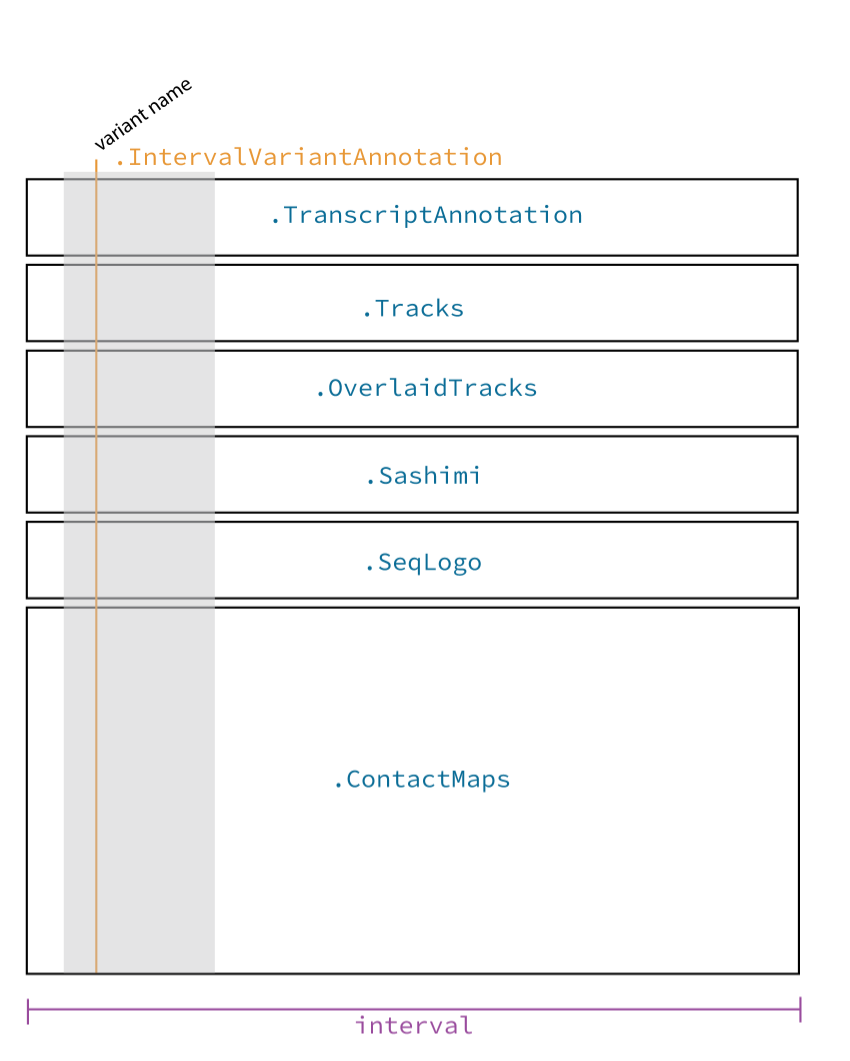
Anatomy of a plot_components.plot figure. Blue labels show component and annotation classes; purple labels show plot() arguments that control figure-wide layout.

Components and annotations

Each component class wraps a model output container (or custom data placed in TrackData, GeneExpressionData, or JunctionData) and controls panel-level aesthetics such as colors, y-axis scaling (shared_y_scale, global_ylims), and y-axis label templates (ylabel_template).

Class	Input container	Recommended outputs	Description
Tracks	TrackData (1D)	Positional tracks (ATAC, DNASE, RNA_SEQ, CAGE, CHIP_HISTONE, CHIP_TF, SPLICE_SITES, SPLICE_SITE_USAGE; METHYLATION and SC_ATAC in AlphaGenome 2 only; PROCAP in AlphaGenome 1 only)	Line or filled-area profile across genomic coordinates, one subplot per track.
OverlaidTracks	Mapping[str, TrackData]	REF vs. ALT positional tracks	Overlays two or more TrackData objects with matching metadata on the same axes to compare variant alleles or conditions.
GeneExpression	GeneExpressionData	SC_GENE_EXPRESSION_DENOISED, SC_GENE_EXPRESSION (AlphaGenome 2 only)	Horizontal gene-span bars showing scalar gene-level expression (in CPM, or log1p with log_scale=True) across genes overlapping the interval.
OverlaidGeneExpression	Mapping[str, GeneExpressionData]	REF vs. ALT gene-level expression (AlphaGenome 2 only)	Overlays two or more GeneExpressionData objects on the same axes to compare REF and ALT gene expression across an interval.
Sashimi	JunctionData	SPLICE_JUNCTIONS	Arcs connecting splice donor and acceptor coordinates, with arc thickness and optional labels showing normalized junction read counts.
EnhancerArcs	DataFrame	Enhancer-to-gene links from get_active_enhancers() (AlphaGenome 2 only)	Cubic Bezier arcs connecting candidate enhancer intervals to target gene TSS coordinates, optionally colored or scaled by enhancer score.
ContactMaps	TrackData (2D)	CONTACT_MAPS	Pairwise 2D heatmap of chromatin contact frequencies across genomic bins.
ContactMapsDiff	TrackData (2D)	ALT - REF CONTACT_MAPS	Pairwise 2D heatmap with a zero-centered diverging colormap (RdBu_r) for contact map differences.
SeqLogo	np.ndarray (S, A) + Interval	ISM contribution scores	Nucleotide sequence logo where letter heights reflect per-base attribution or in silico mutagenesis scores.
TranscriptAnnotation	Sequence[Transcript]	GENCODE / GTF transcripts	Horizontal gene and isoform models showing exons, introns, coding regions, and strand direction.
VariantAnnotation	Sequence[Variant]	Variant positions	Vertical highlight lines spanning all panels at each variant coordinate, with optional angled labels at the top of the figure.
IntervalAnnotation	Sequence[Interval]	Candidate regulatory elements, exons, or ROIs	Shaded vertical bands spanning all panels across each genomic interval, with optional labels.

Custom components

To define a custom panel type or cross-panel overlay, subclass AbstractComponent (implementing num_axes, get_ax_height, and plot_ax) or AbstractAnnotation (implementing plot_ax and plot_labels).