Analyzing a splicing variant

Analyzing a splicing variant#

Variants can alter how a gene is spliced, not only how much it is expressed. This tutorial uses AlphaGenome 2 to predict, visualize, and score a splicing variant: chr22:36201698:A>C at APOL4 in sigmoid colon (UBERON:0001159), an example highlighted in the AlphaGenome 1 quick start (legacy) and Avsec et al. [2026].

Key activities:

Inspect how AlphaGenome 2 represents splicing outputs and verify their measurement status in sigmoid colon.
Predict REF and ALT tracks for RNA_SEQ, SPLICE_SITES, SPLICE_SITE_USAGE, and SPLICE_JUNCTIONS.
Plot negative-strand junction arcs (plot_components.Sashimi) alongside overlaid splice site usage and RNA-seq coverage.
Score the variant across the recommended splicing and RNA-seq variant scorers.

Set up#

# @title Install AlphaGenome

# @markdown Run this cell to install AlphaGenome.
from IPython.display import clear_output
! pip install alphagenome
clear_output()

# @title Imports
from alphagenome import colab_utils
from alphagenome.data import gene_annotation
from alphagenome.data import genome
from alphagenome.data import transcript as transcript_utils
from alphagenome.models.v2 import dna_client
from alphagenome.models.v2 import variant_scorers
from alphagenome.visualization import plot_components
import matplotlib.pyplot as plt
import pandas as pd

Store your API key in Colab Secrets for persistent access across sessions (see Installation), then initialize the client:

dna_model = dna_client.create(colab_utils.get_api_key())

Splicing outputs#

AlphaGenome 2 predicts splicing with three specialized output types, alongside bulk RNA-seq coverage, which also captures splicing patterns (see Model output metadata):

Output type	Resolution	Description
`SPLICE_SITES`	1 bp	Condition-specific classification probabilities across 5 channels (donor and acceptor on each strand plus non-splice-site padding), derived per condition from its RNA-seq splicing assays.
`SPLICE_SITE_USAGE`	1 bp	Condition-specific fraction of transcripts spliced at each donor or acceptor site per RNA-seq track.
`SPLICE_JUNCTIONS`	Junction pairs	Condition-specific split-read counts spanning donor-acceptor intron pairs.

Check the imputation_mode status of RNA_SEQ and the three splicing output types in sigmoid colon (UBERON:0001159) via dna_model.supported_conditions():

condition = 'UBERON:0001159'  # Sigmoid colon.

dna_model.supported_conditions().set_index('condition').loc[
    condition,
    ['rna_seq', 'splice_sites', 'splice_site_usage', 'splice_junctions'],
]

rna_seq              observed
splice_sites         observed
splice_site_usage    observed
splice_junctions     observed
Name: UBERON:0001159, dtype: object

Load GENCODE gene annotations and construct a TranscriptExtractor across all protein-coding transcripts (rather than restricting to MANE Select alone) so alternative APOL4 isoforms are displayed:

gtf = pd.read_feather(
    'https://storage.googleapis.com/alphagenome/reference/gencode/'
    'hg38/gencode.v46.annotation.gtf.gz.feather'
)
gtf_transcripts = gene_annotation.filter_protein_coding(gtf)
transcript_extractor = transcript_utils.TranscriptExtractor(gtf_transcripts)

Predict the variant#

Center a 1 Mb sequence window (dna_client.SEQUENCE_LENGTH_1MB) around chr22:36201698:A>C (genome.Variant) and predict RNA_SEQ, SPLICE_SITES, SPLICE_SITE_USAGE, and SPLICE_JUNCTIONS for both REF and ALT alleles:

variant = genome.Variant(
    chromosome='chr22',
    position=36201698,
    reference_bases='A',
    alternate_bases='C',
)
interval = variant.reference_interval.resize(dna_client.SEQUENCE_LENGTH_1MB)

output = dna_model.predict_variant(
    interval=interval,
    variant=variant,
    requested_outputs=[
        dna_client.OutputType.RNA_SEQ,
        dna_client.OutputType.SPLICE_SITES,
        dna_client.OutputType.SPLICE_SITE_USAGE,
        dna_client.OutputType.SPLICE_JUNCTIONS,
    ],
    condition=condition,
)

Visualize splicing and expression changes#

We keep observed negative-strand GTEx tracks (output.reference.filter_to_observed()) and plot REF and ALT junction arcs (plot_components.Sashimi), splice site usage, and RNA-seq coverage across APOL4:

plot_interval = gene_annotation.get_gene_interval(gtf, gene_symbol='APOL4').pad(
    1000, 1000
)
obs_ref = output.reference.filter_to_observed()
obs_alt = output.alternate.filter_to_observed()

ref_j = obs_ref.splice_junctions.filter_to_strand('-')
alt_j = obs_alt.splice_junctions.filter_to_strand('-')
gtex_j_mask = (ref_j.metadata['data_source'] == 'gtex').values

ref_ssu = obs_ref.splice_site_usage.filter_to_negative_strand().slice_by_interval(
    plot_interval, match_resolution=True
)
alt_ssu = obs_alt.splice_site_usage.filter_to_negative_strand().slice_by_interval(
    plot_interval, match_resolution=True
)
gtex_ssu_mask = (ref_ssu.metadata['data_source'] == 'gtex').values

ref_rna = obs_ref.rna_seq.filter_to_negative_strand().slice_by_interval(
    plot_interval, match_resolution=True
)
alt_rna = obs_alt.rna_seq.filter_to_negative_strand().slice_by_interval(
    plot_interval, match_resolution=True
)
rna_mask = (
    (ref_rna.metadata['Assay title'] == 'polyA plus RNA-seq')
    & (ref_rna.metadata['endedness'] == 'paired')
).values

transcripts = transcript_extractor.extract(interval)
ref_alt_colors = {'REF': '#22AAE1', 'ALT': 'red'}

plot_components.plot(
    [
        plot_components.TranscriptAnnotation(transcripts),
        plot_components.Sashimi(
            ref_j.filter_tracks(gtex_j_mask),
            ylabel_template='REF junctions ({strand})\n{biosample_name}',
        ),
        plot_components.Sashimi(
            alt_j.filter_tracks(gtex_j_mask),
            ylabel_template='ALT junctions ({strand})\n{biosample_name}',
        ),
        plot_components.OverlaidTracks(
            tdata={
                'REF': ref_ssu.filter_tracks(gtex_ssu_mask),
                'ALT': alt_ssu.filter_tracks(gtex_ssu_mask),
            },
            colors=ref_alt_colors,
            ylabel_template='Splice site usage ({strand})\n{biosample_name}',
        ),
        plot_components.OverlaidTracks(
            tdata={
                'REF': ref_rna.filter_tracks(rna_mask),
                'ALT': alt_rna.filter_tracks(rna_mask),
            },
            colors=ref_alt_colors,
            ylabel_template='RNA-seq ({strand})\n{biosample_name}',
        ),
    ],
    interval=plot_interval,
    annotations=[plot_components.VariantAnnotation([variant], alpha=0.8)],
)
plt.show()

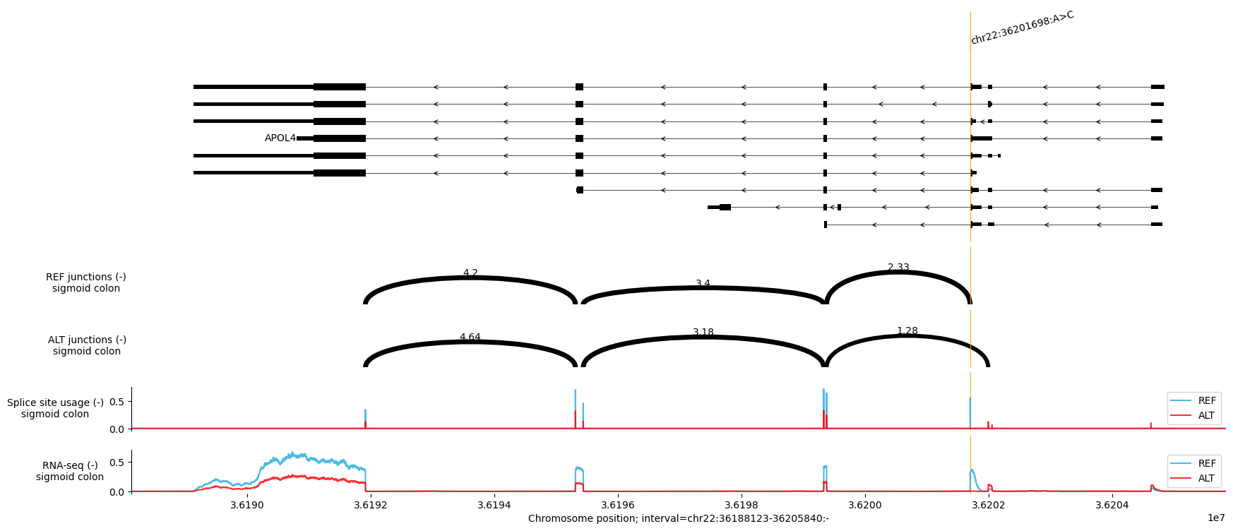
../../_images/3014094ede0595492e8bc984b15ac332a4acd0df8c96a44e0486eedd9868c56b.png

On the negative strand at APOL4, AlphaGenome 2 predicts that the ALT allele (C at chr22:36201698) suppresses the canonical splice junction adjacent to the variant, shifts split reads toward an upstream exon-skipping junction, reduces predicted donor splice-site usage at the disrupted exon boundary, and lowers exon RNA-seq coverage across APOL4.

Score the variant#

Quantify these effects across all three splicing scorers (SPLICE_SITES, SPLICE_SITE_USAGE, SPLICE_JUNCTIONS) together with RNA_SEQ from variant_scorers.RECOMMENDED_VARIANT_SCORERS, then format the per-gene results with variant_scorers.tidy_scores:

splicing_scorers = [
    variant_scorers.RECOMMENDED_VARIANT_SCORERS[name]
    for name in ('SPLICE_SITES', 'SPLICE_SITE_USAGE', 'SPLICE_JUNCTIONS')
]
scores = dna_model.score_variant(
    interval=interval,
    variant=variant,
    variant_scorers=[
        *splicing_scorers,
        variant_scorers.RECOMMENDED_VARIANT_SCORERS['RNA_SEQ'],
    ],
    condition=condition,
)
tidy = variant_scorers.tidy_scores(scores, match_gene_strand=True)
tidy[tidy['gene_name'] == 'APOL4']

	variant_id	scored_interval	gene_id	gene_name	gene_type	gene_strand	junction_Start	junction_End	output_type	variant_scorer	track_name	track_strand	imputation_mode	biosample_curie	biosample_type	biosample_name	splice_site_type	Assay title	data_source	data_pipeline	genetically_modified	endedness	raw_score
0	chr22:36201698:A>C	chr22:35677410-36725986:.	ENSG00000100336	APOL4	protein_coding	-	None	None	SPLICE_SITES	GeneMaskSplicingScorer(requested_output=SPLICE_SITES, width=None)	UBERON:0001159_donor	.	observed	UBERON:0001159	tissue	sigmoid colon	donor	NaN	NaN	NaN	NaN	NaN	0.895063
1	chr22:36201698:A>C	chr22:35677410-36725986:.	ENSG00000100336	APOL4	protein_coding	-	None	None	SPLICE_SITES	GeneMaskSplicingScorer(requested_output=SPLICE_SITES, width=None)	UBERON:0001159_acceptor	.	observed	UBERON:0001159	tissue	sigmoid colon	acceptor	NaN	NaN	NaN	NaN	NaN	0.255946
2	chr22:36201698:A>C	chr22:35677410-36725986:.	ENSG00000100336	APOL4	protein_coding	-	None	None	SPLICE_SITE_USAGE	GeneMaskSplicingScorer(requested_output=SPLICE_SITE_USAGE, width=None)	UBERON:0001159_polyA plus RNA-seq-encode	.	observed	UBERON:0001159	tissue	sigmoid colon	NaN	polyA plus RNA-seq	encode	encode	NaN	NaN	0.593331
3	chr22:36201698:A>C	chr22:35677410-36725986:.	ENSG00000100336	APOL4	protein_coding	-	None	None	SPLICE_SITE_USAGE	GeneMaskSplicingScorer(requested_output=SPLICE_SITE_USAGE, width=None)	UBERON:0001159_polyA plus RNA-seq-gtex	.	observed	UBERON:0001159	tissue	sigmoid colon	NaN	polyA plus RNA-seq	gtex	recount3	NaN	NaN	0.556729
4	chr22:36201698:A>C	chr22:35677410-36725986:.	ENSG00000100336	APOL4	protein_coding	-	None	None	SPLICE_SITE_USAGE	GeneMaskSplicingScorer(requested_output=SPLICE_SITE_USAGE, width=None)	UBERON:0001159_total RNA-seq-encode	.	observed	UBERON:0001159	tissue	sigmoid colon	NaN	total RNA-seq	encode	encode	NaN	NaN	0.566698
5	chr22:36201698:A>C	chr22:35677410-36725986:.	ENSG00000100336	APOL4	protein_coding	-	36199376	36201699	SPLICE_JUNCTIONS	SpliceJunctionScorer()	UBERON:0001159_polyA plus RNA-seq-encode	.	observed	UBERON:0001159	tissue	sigmoid colon	NaN	polyA plus RNA-seq	encode	encode	NaN	NaN	5.640625
6	chr22:36201698:A>C	chr22:35677410-36725986:.	ENSG00000100336	APOL4	protein_coding	-	36199376	36201699	SPLICE_JUNCTIONS	SpliceJunctionScorer()	UBERON:0001159_polyA plus RNA-seq-gtex	.	observed	UBERON:0001159	tissue	sigmoid colon	NaN	polyA plus RNA-seq	gtex	recount3	NaN	NaN	5.792969
7	chr22:36201698:A>C	chr22:35677410-36725986:.	ENSG00000100336	APOL4	protein_coding	-	36199376	36201699	SPLICE_JUNCTIONS	SpliceJunctionScorer()	UBERON:0001159_total RNA-seq-encode	.	observed	UBERON:0001159	tissue	sigmoid colon	NaN	total RNA-seq	encode	encode	NaN	NaN	5.699219
13	chr22:36201698:A>C	chr22:35677410-36725986:.	ENSG00000100336	APOL4	protein_coding	-	None	None	RNA_SEQ	GeneMaskLFCScorer(requested_output=RNA_SEQ, aggregation_type=DIFF_MEAN)	UBERON:0001159_polyA plus RNA-seq-encode-paired-ended	.	observed	UBERON:0001159	tissue	sigmoid colon	NaN	polyA plus RNA-seq	encode	encode	False	paired	-0.893399
14	chr22:36201698:A>C	chr22:35677410-36725986:.	ENSG00000100336	APOL4	protein_coding	-	None	None	RNA_SEQ	GeneMaskLFCScorer(requested_output=RNA_SEQ, aggregation_type=DIFF_MEAN)	UBERON:0001159_polyA plus RNA-seq-encode-single-ended	.	imputed_supported	UBERON:0001159	tissue	sigmoid colon	NaN	polyA plus RNA-seq	NaN	encode	NaN	single	-1.041781
15	chr22:36201698:A>C	chr22:35677410-36725986:.	ENSG00000100336	APOL4	protein_coding	-	None	None	RNA_SEQ	GeneMaskLFCScorer(requested_output=RNA_SEQ, aggregation_type=DIFF_MEAN)	UBERON:0001159_total RNA-seq-encode-paired-ended	.	observed	UBERON:0001159	tissue	sigmoid colon	NaN	total RNA-seq	encode	encode	False	paired	-1.595810
16	chr22:36201698:A>C	chr22:35677410-36725986:.	ENSG00000100336	APOL4	protein_coding	-	None	None	RNA_SEQ	GeneMaskLFCScorer(requested_output=RNA_SEQ, aggregation_type=DIFF_MEAN)	UBERON:0001159_total RNA-seq-encode-single-ended	.	imputed_supported	UBERON:0001159	tissue	sigmoid colon	NaN	total RNA-seq	NaN	encode	NaN	single	-1.391649
17	chr22:36201698:A>C	chr22:35677410-36725986:.	ENSG00000100336	APOL4	protein_coding	-	None	None	RNA_SEQ	GeneMaskLFCScorer(requested_output=RNA_SEQ, aggregation_type=DIFF_MEAN)	UBERON:0001159_polyA plus RNA-seq-gtex-paired-ended	.	observed	UBERON:0001159	tissue	sigmoid colon	NaN	polyA plus RNA-seq	gtex	recount3	False	paired	-1.349591

Combine the splicing scores#

Following the splicing variant benchmarks in Avsec et al. [2026], we can combine the maximum magnitude across genes and observed tracks for each of the three splicing output types into a single merged splicing score per variant:

\[\text{alphagenome\_splicing} = \max|\text{splice\_sites}| + \max|\text{splice\_site\_usage}| + \frac{\max|\text{splice\_junctions}|}{5}\]

Giving weight 0.2 (1 / 5) to SPLICE_JUNCTIONS accounts for the larger scale of junction log-fold changes relative to probability differences ([0, 1]).

Note

Multi-tissue ensembling: Each AlphaGenome 2 call scores one condition at a time. In AlphaGenome 1 (alphagenome.models.v1), score_variant evaluates all observed biosamples simultaneously; scoring or taking the maximum across multiple relevant tissues can improve sensitivity for tissue-restricted splice variants.
Imputed splicing tracks: Filter to imputation_mode == "observed" when available, as imputed SPLICE_SITE_USAGE and SPLICE_JUNCTIONS tracks carry additional caveats; see Navigating imputed tracks.

def compute_merged_splicing_score(df: pd.DataFrame) -> pd.DataFrame:
  """Computes the merged splicing score across observed tracks per variant."""
  obs_df = df[df['imputation_mode'] == 'observed'].copy()
  obs_df['variant_id'] = obs_df['variant_id'].map(str)
  obs_df['abs_raw_score'] = obs_df['raw_score'].abs()
  max_scores = (
      obs_df.groupby(['variant_id', 'output_type'])['abs_raw_score']
      .max()
      .reset_index()
      .pivot(index='variant_id', columns='output_type', values='abs_raw_score')
      .fillna(0.0)
  )
  max_scores['alphagenome_splicing'] = (
      max_scores.get('SPLICE_SITES', 0.0)
      + max_scores.get('SPLICE_SITE_USAGE', 0.0)
      + max_scores.get('SPLICE_JUNCTIONS', 0.0) / 5.0
  )
  return max_scores.reset_index()


compute_merged_splicing_score(tidy)

output_type	variant_id	RNA_SEQ	SPLICE_JUNCTIONS	SPLICE_SITES	SPLICE_SITE_USAGE	alphagenome_splicing
0	chr22:36201698:A>C	1.59581	5.792969	0.895063	0.593331	2.646988

Next steps#

See Deriving PSI values from splice junctions to compute percent spliced in (PSI5 and PSI3) ratios from JunctionData predictions.
Explore additional track and junction plotting layouts in Plotting predictions.
Read How variant scoring works for details on spatial aggregation and gene masks across scorers.