Plotting predictions

The plot_components module builds a figure from a list of panels stacked over a shared genomic interval. Pass the panels and the interval to plot_components.plot, which returns a matplotlib figure you can save with fig.savefig.

Panels fall into two groups:

• Annotations mark genes, variants, and other intervals: TranscriptAnnotation, VariantAnnotation, and IntervalAnnotation.

• Data panels show predictions: Tracks for coverage, GeneExpression for gene-level single-cell expression, Sashimi for splice junctions, and ContactMaps for 3D contacts. Overlaid versions compare REF and ALT alleles on the same axes.

Track labels are built from track metadata with ylabel_template, for example '{biosample_name} ({strand})'.

For variant overlays and splice junction arcs in context, see Predicting a variant and Analyzing a splicing variant. The Visualization API reference lists every component and parameter.

Set up

# @title Install AlphaGenome

# @markdown Run this cell to install AlphaGenome.
from IPython.display import clear_output
! pip install alphagenome
clear_output()

Store your API key in Colab Secrets for persistent access across sessions (see Installation).

from alphagenome import colab_utils
from alphagenome.data import gene_annotation, gene_expression_data, genome, track_data, transcript
from alphagenome.models.v2 import dna_client
from alphagenome.visualization import plot_components
import matplotlib.pyplot as plt
import numpy as np
import pandas as pd

Load model and auxiliary objects

dna_model = dna_client.create(colab_utils.get_api_key())

# Load observed metadata objects for human.
output_metadata = dna_model.observed_metadata(
    organism=dna_client.Organism.HOMO_SAPIENS
)

# Load gene annotations (from GENCODE).
gtf = pd.read_feather(
    'https://storage.googleapis.com/alphagenome/reference/gencode/'
    'hg38/gencode.v46.annotation.gtf.gz.feather'
)

# Filter to protein-coding genes and highly supported transcripts.
gtf_transcript = gene_annotation.filter_transcript_support_level(
    gene_annotation.filter_protein_coding(gtf), ['1']
)

# Extractor for identifying transcripts in a region.
transcript_extractor = transcript.TranscriptExtractor(gtf_transcript)

# Also define an extractor that fetches only the longest transcript per gene.
gtf_longest_transcript = gene_annotation.filter_to_longest_transcript(
    gtf_transcript
)
longest_transcript_extractor = transcript.TranscriptExtractor(
    gtf_longest_transcript
)

RNA-seq and CAGE coverage

RNA_SEQ and CAGE are coverage tracks that measure gene expression signal. We predict RNA_SEQ and CAGE in sigmoid colon tissue for a genomic interval containing APOL4. Positions of the longest transcript per gene in this interval are shown at the top:

# Define interval to make predictions for (used throughout this tutorial).
# Note that the interval width must be one of the supported sequence lengths.
interval = genome.Interval('chr22', 36_150_498, 36_252_898).resize(
    dna_client.SEQUENCE_LENGTH_1MB
)

# Define the tissue/cell-type to predict expression for.
condition = 'UBERON:0001159'  # Colon - Sigmoid

# Make predictions.
output = dna_model.predict_interval(
    interval=interval,
    requested_outputs={
        dna_client.OutputType.RNA_SEQ,
        dna_client.OutputType.CAGE,
    },
    condition=condition,
)
# Extract the longest transcripts per gene for this interval.
longest_transcripts = longest_transcript_extractor.extract(interval)

Pass a list of panels to plot_components.plot:

# Build plot.
plot = plot_components.plot(
    [
        plot_components.TranscriptAnnotation(longest_transcripts),
        plot_components.Tracks(
            tdata=output.rna_seq,
            ylabel_template='RNA_SEQ: {biosample_name} ({strand})\n{name}',
        ),
        plot_components.Tracks(
            tdata=output.cage,
            ylabel_template='CAGE: {biosample_name} ({strand})\n{name}',
        ),
    ],
    interval=interval,
    title='Predicted RNA Expression (RNA_SEQ, CAGE) for colon tissue',
)

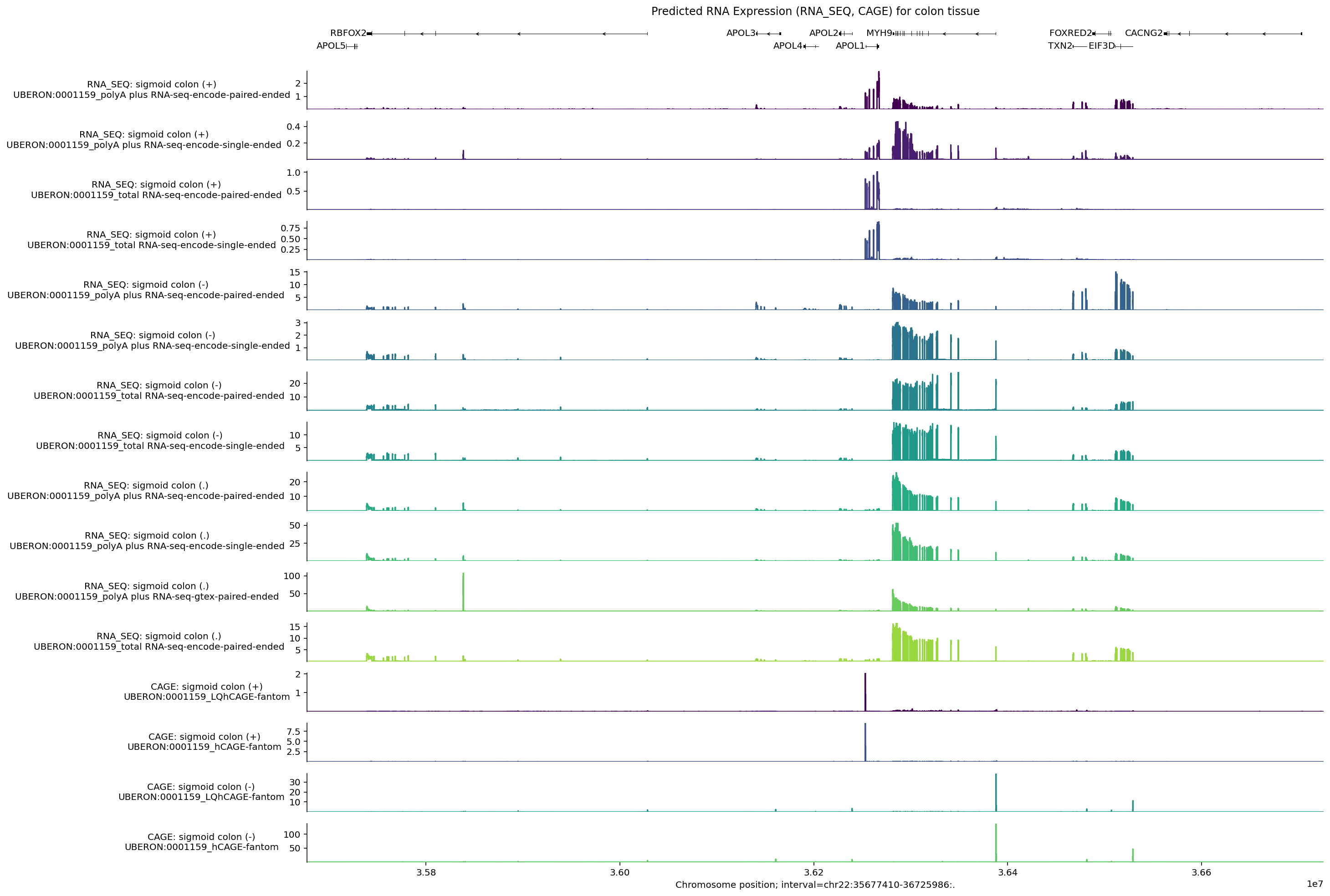
Note that the positive and negative stranded tracks have clearly different signals. Let’s check which genes are transcribed from the positive strand:

[t.info['gene_name'] for t in longest_transcripts if t.strand == '+']

['APOL5', 'APOL1']

For both positive-strand RNA_SEQ tracks, RNA-seq coverage is highest across APOL1. Similarly for CAGE, positive-strand peaks fall near the start of APOL1, whereas APOL5 shows no peaks because it is not expressed in colon tissue (GTEx).

Zoom in and customize track labels

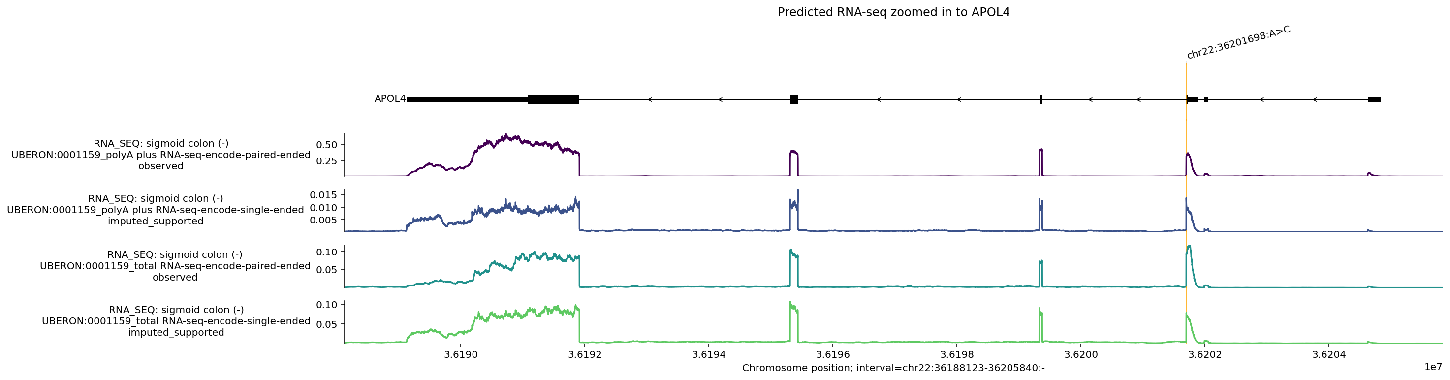
The model predicts across the full 1 Mb input window, while interval= in plot_components.plot controls the plotted window. Including {imputation_mode} in ylabel_template indicates whether each track was directly measured (observed) or imputed in the target condition:

apol4_interval = gene_annotation.get_gene_interval(gtf, gene_symbol='APOL4')
apol4_interval = apol4_interval.resize(apol4_interval.width + 2000)
transcripts = transcript_extractor.extract(interval)

variant = genome.Variant.from_str('chr22_36201698_A_C', genome.VariantFormat.GTEX)

fig = plot_components.plot(
    [
        plot_components.TranscriptAnnotation(longest_transcripts),
        plot_components.Tracks(
            tdata=output.rna_seq.filter_to_negative_strand(),
            ylabel_template=(
                'RNA_SEQ: {biosample_name} ({strand})\n{name}\n{imputation_mode}'
            ),
        ),
    ],
    interval=apol4_interval,
    annotations=[plot_components.VariantAnnotation([variant])],
    title='Predicted RNA-seq zoomed in to APOL4',
)
plt.show()

Plot custom annotation (e.g., polyadenylation sites)

# Run predictions with an additional ontology to highlight differences across
# tissues.
conditions = [
    'UBERON:0001159',  # Colon - Sigmoid.
    'UBERON:0002048',  # lung.
]

# Make predictions.
outputs = [
    dna_model.predict_interval(
        interval=interval,
        requested_outputs={
            dna_client.OutputType.RNA_SEQ,
        },
        condition=condition,
    )
    for condition in conditions
]

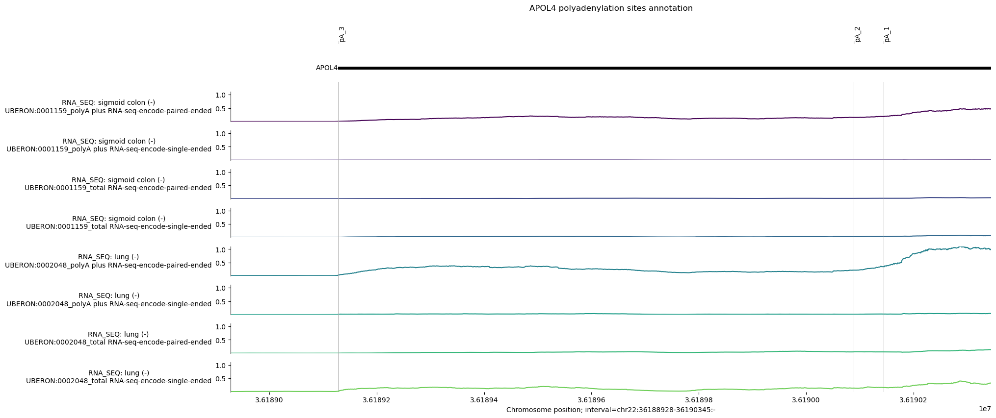
There are 3 annotated polyadenylation (pA) sites overlapping APOL4 transcripts from PolyADBv3 (Wang et al. 2018). We define these positions as 1 bp intervals in hg38 coordinates:

# Define pA sites in hg38 coordinates.
apol4_pAs = [
    genome.Interval('chr22', 36_189_128, 36_189_129, '-'),
    genome.Interval('chr22', 36_190_089, 36_190_090, '-'),
    genome.Interval('chr22', 36_190_144, 36_190_145, '-'),
]

# Define plotting interval as first/last pA plus some offset distance.

offset = 200
pA_interval = genome.Interval(
    'chr22', 36_189_128 - offset, 36_190_145 + offset, '-'
)

# Define intervals annotation.
pA_labels = ['pA_3', 'pA_2', 'pA_1']

# Build plot.
# NOTE: Depending on annotation distance and interval zoom, some annotations may
# appear as overlapping.

plot = plot_components.plot(
    [
        plot_components.TranscriptAnnotation(longest_transcripts),
        # RNA-seq tracks.
        plot_components.Tracks(
            tdata=track_data.concat([
                output.rna_seq.filter_to_negative_strand() for output in outputs
            ]),
            ylabel_template='RNA_SEQ: {biosample_name} ({strand})\n{name}',
            shared_y_scale=True,
        ),
    ],
    annotations=[
        plot_components.IntervalAnnotation(
            apol4_pAs, alpha=1, labels=pA_labels, label_angle=90
        )
    ],
    interval=pA_interval,
    title='APOL4 polyadenylation sites annotation',
)

Single-cell gene expression

For single-cell data, AlphaGenome 2 outputs a predicted expression value per gene rather than a base-resolution coverage track.

To show gene-level values alongside coverage tracks, GeneExpression draws each gene’s predicted value as a horizontal segment over the gene body labeled in counts per million (CPM). Here we compare placental epithelial cells, which express APOL4, with placental T cells:

conditions = [
    'UBERON:0001987_CL:0000066',  # Placenta Epithelial Cell
    'UBERON:0001987_CL:0000084',  # Placenta T-cell
]

output = [
    dna_model.predict_interval(
        interval=interval,
        requested_outputs={
            dna_client.OutputType.SC_GENE_EXPRESSION,
        },
        condition=condition,
    )
    for condition in conditions
]

For SC_GENE_EXPRESSION, predictions are returned as GeneExpressionData objects containing a gene-by-track values matrix alongside gene_metadata and track_metadata tables. Convenience methods (filter_to_protein_coding(), filter_to_observed(), filter_to_negative_strand()) or boolean masks filter to genes and tracks of interest.

As with track_data.concat for TrackData, use gene_expression_data.concat to combine predictions from multiple conditions:

# Concatenate predictions for the two queried ontologies
gex_pred = gene_expression_data.concat(
    [out.sc_gene_expression for out in output]
)

# Select only protein-coding genes and observed, negative strand tracks.
gex_pred = (
    gex_pred.filter_to_protein_coding()
    .filter_to_observed()
    .filter_to_negative_strand()
)

We can now use the GeneExpression component to plot the predicted gene expression values.

Tip

To hide printed CPM labels on each gene bar, pass show_value=False. Setting log_scale=True displays expression on a log1p scale so highly expressed neighbor genes do not compress moderate-expression genes near zero.

plot_components.plot(
    [
        plot_components.TranscriptAnnotation(longest_transcripts),
        plot_components.GeneExpression(
            gdata=gex_pred,
            ylabel_template='{biosample_name} {strand}',
            cmap='RdBu',
            log_scale=True,
            shared_y_scale=True,
        ),
    ],
    interval=interval.resize(100_000),  # We zoom in on APOL4
)
plt.show()

As expected, we observe higher expression of APOL4 in placental epithelial cells than in T cells, and the opposite pattern for APOL3.

Chromatin accessibility

Chromatin accessibility is captured by the DNASE, ATAC, and SC_ATAC output types. We show ATAC and DNASE here (SC_ATAC can be requested the same way), plotting predictions across intestinal tract reference conditions for the interval around APOL4:

# List of IDs corresponding to various intestinal tissues.
conditions = [
    'UBERON:0000317',
    'UBERON:0001155',
    'UBERON:0001157',
    'UBERON:0001159',
    'UBERON:0004992',
    'UBERON:0008971',
]

# Make predictions.
outputs = [
    dna_model.predict_interval(
        interval,
        requested_outputs={
            dna_client.OutputType.DNASE,
            dna_client.OutputType.ATAC,
        },
        condition=condition,
    )
    for condition in conditions
]

Use plot_components.IntervalAnnotation to mark two putative promoters from the Ensembl Regulatory Build and check whether they overlap predicted accessible regions:

# Two putative promoter intervals from Ensembl.
promoter_intervals = [
    genome.Interval(
        'chr22', 36_201_799, 36_202_681, name='Ensembl_promoter:ENSR00001367790'
    ),
    genome.Interval(
        'chr22', 36_204_705, 36_205_330, name='Ensembl_promoter:ENSR00001367792'
    ),
]

# Build plot.
plot = plot_components.plot(
    [
        plot_components.TranscriptAnnotation(longest_transcripts),
        plot_components.Tracks(
            tdata=track_data.concat([output.dnase for output in outputs]),
            ylabel_template='DNASE: {biosample_name} ({strand})\n{name}',
        ),
        plot_components.Tracks(
            tdata=track_data.concat([output.atac for output in outputs]),
            ylabel_template='ATAC: {biosample_name} ({strand})\n{name}',
        ),
    ],
    # Plot an 8kb window around the variant.
    interval=variant.reference_interval.resize(8000),
    annotations=[
        plot_components.VariantAnnotation([variant]),
        plot_components.IntervalAnnotation(promoter_intervals),
    ],
    title='Predicted chromatin accessibility (DNASE, ATAC) for colon tissue',
)

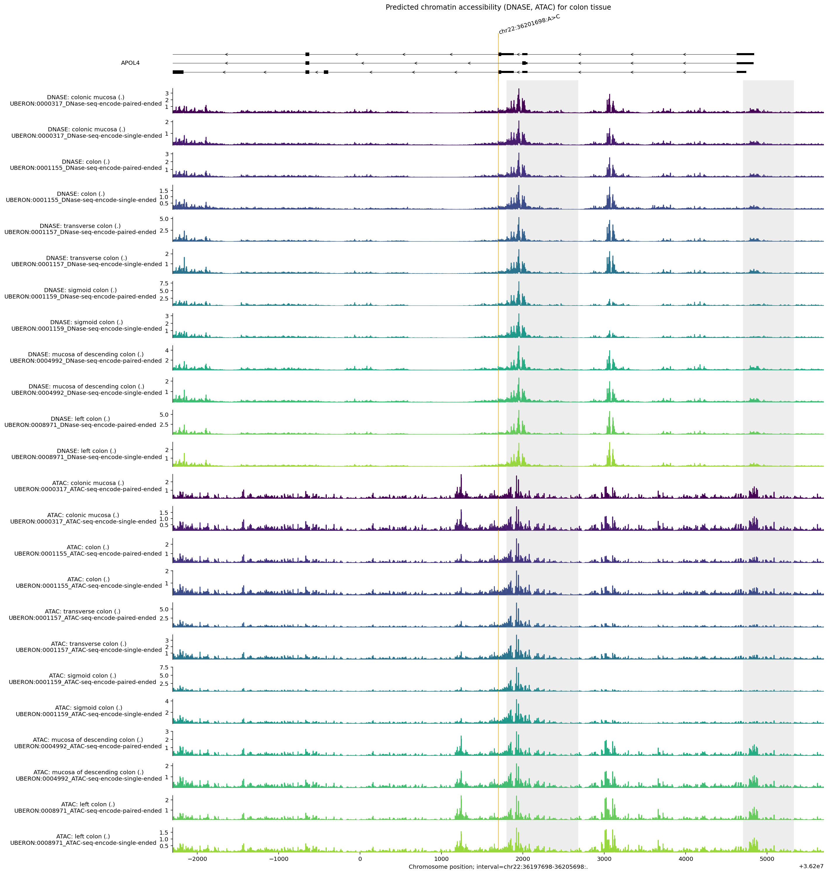
Observations from this plot:

• Elevated DNASE and ATAC signals overlap both putative promoter regions highlighted in grey, and additional accessibility peaks mark candidate distal regulatory elements.

• DNASE and ATAC signals are similar but not identical, reflecting differences in assay protocol.

• Accessibility is low directly at the variant position (orange line).

Histone ChIP-seq

Histone modification marks are captured by the CHIP_HISTONE output. Here we visualize predictions across the same interval for colon tissues.

Two properties apply to CHIP_HISTONE (and CHIP_TF) predictions in AlphaGenome 2:

• Predictions are returned at 128 bp resolution, and plot_components aligns plotted intervals to bin boundaries automatically.

• Every supported condition returns all 43 histone ChIP channels (covering 32 marks split by sequencing endedness). Use dna_model.observed_metadata(...) or metadata['imputation_mode'] to inspect which histone marks were directly measured (observed) in each tissue:

output_metadata.chip_histone[
    output_metadata.chip_histone['biosample_name'].str.contains('colon')
]

	name	strand	biosample_curie	imputation_mode	biosample_type	biosample_name	Assay title	data_source	histone_mark	genetically_modified	endedness	data_pipeline
191	UBERON:0000317_Histone ChIP-seq-encode-H3K27ac...	.	UBERON:0000317	observed	tissue	colonic mucosa	Histone ChIP-seq	encode	H3K27ac	False	single	encode
192	UBERON:0000317_Histone ChIP-seq-encode-H3K27me...	.	UBERON:0000317	observed	tissue	colonic mucosa	Histone ChIP-seq	encode	H3K27me3	False	single	encode
193	UBERON:0000317_Histone ChIP-seq-encode-H3K36me...	.	UBERON:0000317	observed	tissue	colonic mucosa	Histone ChIP-seq	encode	H3K36me3	False	single	encode
194	UBERON:0000317_Histone ChIP-seq-encode-H3K4me1...	.	UBERON:0000317	observed	tissue	colonic mucosa	Histone ChIP-seq	encode	H3K4me1	False	single	encode
195	UBERON:0000317_Histone ChIP-seq-encode-H3K4me3...	.	UBERON:0000317	observed	tissue	colonic mucosa	Histone ChIP-seq	encode	H3K4me3	False	single	encode
196	UBERON:0000317_Histone ChIP-seq-encode-H3K9ac-...	.	UBERON:0000317	observed	tissue	colonic mucosa	Histone ChIP-seq	encode	H3K9ac	False	single	encode
218	UBERON:0001157_Histone ChIP-seq-encode-H3K27ac...	.	UBERON:0001157	observed	tissue	transverse colon	Histone ChIP-seq	encode	H3K27ac	False	single	encode
219	UBERON:0001157_Histone ChIP-seq-encode-H3K27me...	.	UBERON:0001157	observed	tissue	transverse colon	Histone ChIP-seq	encode	H3K27me3	False	single	encode
220	UBERON:0001157_Histone ChIP-seq-encode-H3K36me...	.	UBERON:0001157	observed	tissue	transverse colon	Histone ChIP-seq	encode	H3K36me3	False	single	encode
221	UBERON:0001157_Histone ChIP-seq-encode-H3K4me1...	.	UBERON:0001157	observed	tissue	transverse colon	Histone ChIP-seq	encode	H3K4me1	False	single	encode
222	UBERON:0001157_Histone ChIP-seq-encode-H3K4me3...	.	UBERON:0001157	observed	tissue	transverse colon	Histone ChIP-seq	encode	H3K4me3	False	single	encode
223	UBERON:0001159_Histone ChIP-seq-encode-H3K27ac...	.	UBERON:0001159	observed	tissue	sigmoid colon	Histone ChIP-seq	encode	H3K27ac	False	single	encode
224	UBERON:0001159_Histone ChIP-seq-encode-H3K27me...	.	UBERON:0001159	observed	tissue	sigmoid colon	Histone ChIP-seq	encode	H3K27me3	False	single	encode
225	UBERON:0001159_Histone ChIP-seq-encode-H3K36me...	.	UBERON:0001159	observed	tissue	sigmoid colon	Histone ChIP-seq	encode	H3K36me3	False	single	encode
226	UBERON:0001159_Histone ChIP-seq-encode-H3K4me1...	.	UBERON:0001159	observed	tissue	sigmoid colon	Histone ChIP-seq	encode	H3K4me1	False	single	encode
227	UBERON:0001159_Histone ChIP-seq-encode-H3K4me3...	.	UBERON:0001159	observed	tissue	sigmoid colon	Histone ChIP-seq	encode	H3K4me3	False	single	encode
303	UBERON:0004992_Histone ChIP-seq-encode-H3K4me1...	.	UBERON:0004992	observed	tissue	mucosa of descending colon	Histone ChIP-seq	encode	H3K4me1	False	single	encode
304	UBERON:0004992_Histone ChIP-seq-encode-H3K4me3...	.	UBERON:0004992	observed	tissue	mucosa of descending colon	Histone ChIP-seq	encode	H3K4me3	False	single	encode
305	UBERON:0004992_Histone ChIP-seq-encode-H3K9me3...	.	UBERON:0004992	observed	tissue	mucosa of descending colon	Histone ChIP-seq	encode	H3K9me3	False	single	encode
1174	UBERON:0012489_Histone ChIP-seq-encode-H3K27ac...	.	UBERON:0012489	observed	tissue	muscle layer of colon	Histone ChIP-seq	encode	H3K27ac	False	single	encode
1175	UBERON:0012489_Histone ChIP-seq-encode-H3K36me...	.	UBERON:0012489	observed	tissue	muscle layer of colon	Histone ChIP-seq	encode	H3K36me3	False	single	encode
1176	UBERON:0012489_Histone ChIP-seq-encode-H3K4me1...	.	UBERON:0012489	observed	tissue	muscle layer of colon	Histone ChIP-seq	encode	H3K4me1	False	single	encode
1177	UBERON:0012489_Histone ChIP-seq-encode-H3K4me3...	.	UBERON:0012489	observed	tissue	muscle layer of colon	Histone ChIP-seq	encode	H3K4me3	False	single	encode
1178	UBERON:0012489_Histone ChIP-seq-encode-H3K9ac-...	.	UBERON:0012489	observed	tissue	muscle layer of colon	Histone ChIP-seq	encode	H3K9ac	False	single	encode

# List of IDs corresponding to various colon tissues in `CHIP_HISTONE` output.
conditions = [
    'UBERON:0000317',
    'UBERON:0001155',
    'UBERON:0001157',
    'UBERON:0001159',
]

# Make predictions.
outputs = [
    dna_model.predict_interval(
        interval=interval,
        requested_outputs={dna_client.OutputType.CHIP_HISTONE},
        condition=condition,
    )
    for condition in conditions
]

We can extract the locations of transcription start sites as annotated by GENCODE using gene_annotation.extract_tss(), and plot these using plot_components.IntervalAnnotation():

gtf_tss = gene_annotation.extract_tss(gtf_longest_transcript)

tss_as_intervals = [
    genome.Interval(
        chromosome=row.Chromosome,
        start=row.Start,
        end=row.End + 1000,  # Add extra 1Kb so the TSSs are visible.
        name=row.gene_name,
    )
    for _, row in gtf_tss.iterrows()
]

We can also reorder tracks so they are grouped by histone mark, and also specify colors based on their histone mark:

concatenated_outputs = track_data.concat(
    [output.chip_histone for output in outputs]
)
reordered_chip_histone = concatenated_outputs.select_tracks_by_index(
    concatenated_outputs.metadata.sort_values('histone_mark').index
)

histone_to_color = {
    'H3K27AC': '#e41a1c',
    'H3K36ME3': '#ff7f00',
    'H3K4ME1': '#377eb8',
    'H3K4ME3': '#984ea3',
    'H3K9AC': '#4daf4a',
    'H3K27ME3': '#ffc0cb',
}
track_colors = (
    reordered_chip_histone.metadata['histone_mark']
    .map(lambda x: histone_to_color.get(x.upper(), '#000000'))
    .values
)

# Build plot.
observed_tracks_mask = (
    reordered_chip_histone.metadata['imputation_mode'] == 'observed'
).values
plot = plot_components.plot(
    [
        plot_components.TranscriptAnnotation(longest_transcripts),
        plot_components.Tracks(
            tdata=reordered_chip_histone.filter_tracks(observed_tracks_mask),
            ylabel_template=(
                'CHIP HISTONE: {biosample_name} ({strand})\n{histone_mark}'
            ),
            filled=True,
            track_colors=track_colors[observed_tracks_mask],
        ),
    ],
    interval=interval,
    annotations=[
        plot_components.IntervalAnnotation(
            tss_as_intervals, alpha=0.5, colors='blue'
        )
    ],
    despine_keep_bottom=True,
    title='Predicted histone modification markers in colon tissue',
)

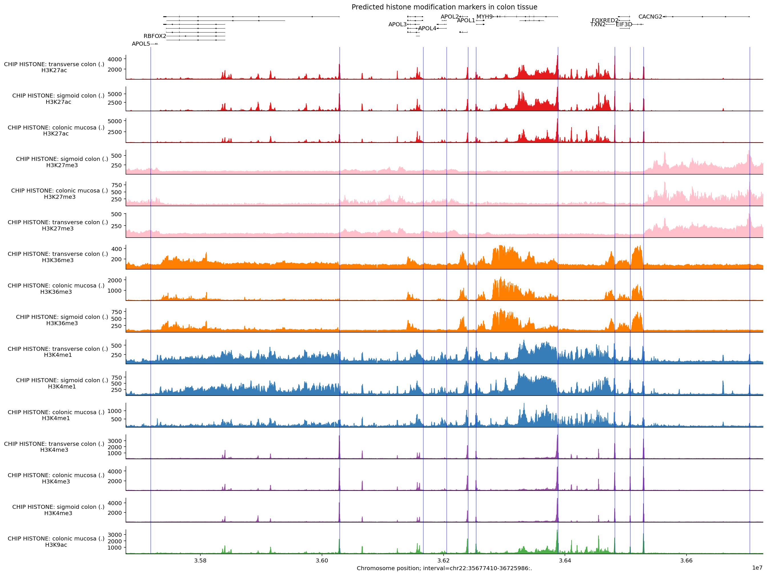
We can see that many of the predicted histone modification peaks overlap with transcription start sites, especially markers associated with promoters (H3K4me3, H3K27ac, and H3K9ac). Other markers such as H3K36me3 and H3K4me1 are more associated with gene bodies and enhancers, so these signals are less pronounced around the TSSs.

TF ChIP-seq

Transcription factor (TF) binding patterns are captured by the CHIP_TF output at 128 bp resolution. Every supported condition returns all 911 TF ChIP channels (covering 778 targets split by sequencing endedness); dna_model.observed_metadata(...) identifies which factors were directly assayed in each biosample (for example, HepG2 and K562 have observed TF ChIP-seq coverage across hundreds of factors).

Here we also demonstrate selecting specific tracks from a TrackData object and aggregating signal across tracks:

conditions = [
    'UBERON:0001159',  # Sigmoid colon.
    'UBERON:0001157',  # Transverse colon.
    'EFO:0002067',  # K562.
    'EFO:0001187',  # HepG2.
]

outputs = [
    dna_model.predict_interval(
        interval=interval,
        requested_outputs={dna_client.OutputType.CHIP_TF},
        condition=condition,
    )
    for condition in conditions
]

concatenated_chip_tf = track_data.concat([output.chip_tf for output in outputs])

Say we then only want to work with the K562 and HepG2 part of the output. We can accomplish this by calling filter_tracks:

conditions = [
    'EFO:0002067',  # K562.
    'EFO:0001187',  # HepG2.
]

output_chip_tf = concatenated_chip_tf.filter_tracks(
    (concatenated_chip_tf.metadata['biosample_curie'].isin(conditions)).values
)
len(output_chip_tf.metadata)

1822

Across the predicted TF ChIP-seq tracks for these two cell lines, maximum predicted values vary substantially across factors:

max_predictions = output_chip_tf.metadata[
    ['biosample_curie', 'biosample_name', 'transcription_factor']
].copy()

max_predictions.loc[:, 'max_prediction'] = output_chip_tf.values.max(axis=0)
max_predictions.sort_values('max_prediction', ascending=False).reset_index(
    drop=True
)

	biosample_curie	biosample_name	transcription_factor	max_prediction
0	EFO:0002067	K562	E2F6	43330.480469
1	EFO:0002067	K562	MAX	34710.921875
2	EFO:0002067	K562	REST	33534.230469
3	EFO:0002067	K562	PKNOX1	33243.894531
4	EFO:0001187	HepG2	REST	32402.304688
...	...	...	...	...
1817	EFO:0002067	K562	GPBP1L1	158.165741
1818	EFO:0002067	K562	BCLAF1	152.707596
1819	EFO:0001187	HepG2	NR0B1	152.435913
1820	EFO:0001187	HepG2	COPS2	151.663513
1821	EFO:0002067	K562	COPS2	145.587006

1822 rows × 4 columns

To keep the multi-track plot legible across 1 Mb, we select only tracks whose maximum predicted peak amplitude exceeds 10_000, which isolates the handful of highest-signal factors in this window:

print(f'Number of tracks before filtering: {len(output_chip_tf.metadata)}')

output_filtered = output_chip_tf.filter_tracks(
    output_chip_tf.values.max(axis=0) > 10_000
)
print(f'Number of tracks after filtering: {len(output_filtered.metadata)}')

Number of tracks before filtering: 1822
Number of tracks after filtering: 23

This is a more manageable number of tracks to visualize. Let’s build up the plot as before:

# Build plot.
plot_components.plot(
    components=[
        plot_components.TranscriptAnnotation(longest_transcripts),
        plot_components.Tracks(
            tdata=output_filtered,
            ylabel_template=(
                'CHIP TF: {biosample_name} ({strand})\n{transcription_factor}'
            ),
            filled=True,
        ),
    ],
    interval=interval,
    title='Predicted TF-binding in K562 and HepG2 cell-lines.',
    despine_keep_bottom=True,
    annotations=[
        plot_components.IntervalAnnotation(
            tss_as_intervals, alpha=0.3, colors='blue'
        )
    ],
)
plt.show()

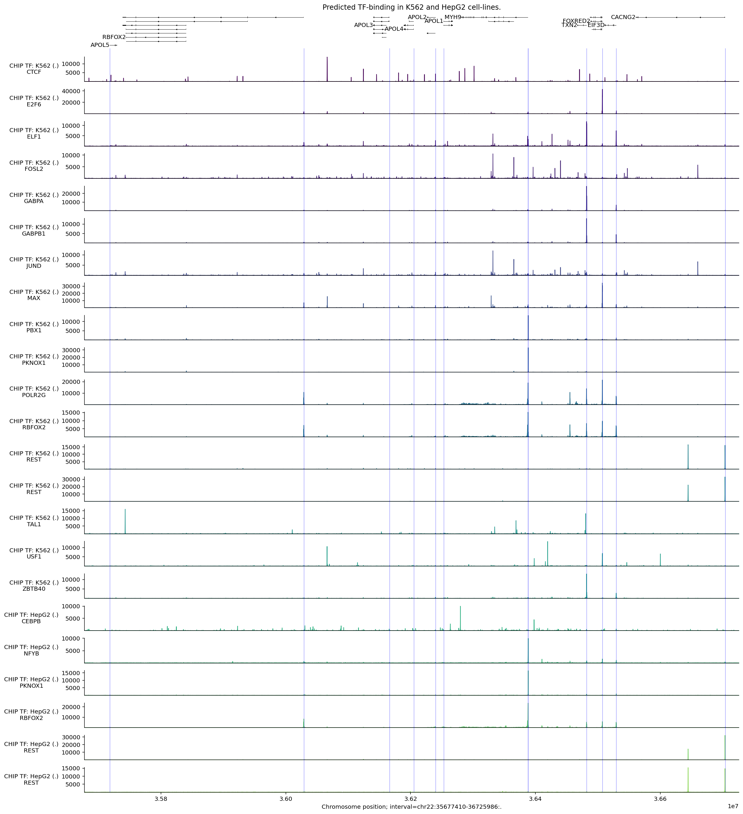
Binding locations for the same protein (e.g., RBFOX2) appear largely the same across these two cell types, with some change in magnitude. Peaks in predicted POLR2G binding, a component of RNA Polymerase II, typically occur near TSS sites.

We can use the same process to select tracks with high peaks anywhere within the APOL4 gene interval:

# Compute max predicted values per track in the APOL4 gene interval.
max_predictions = concatenated_chip_tf.slice_by_interval(
    apol4_interval, match_resolution=True
).values.max(axis=0)

# Filter to the 10 tracks with the highest predictions.
output_filtered = concatenated_chip_tf.filter_tracks(
    (max_predictions >= np.sort(max_predictions)[-10])
)

# Build plot.
plot_components.plot(
    [
        plot_components.TranscriptAnnotation(transcripts),
        plot_components.Tracks(
            tdata=output_filtered,
            ylabel_template=(
                'CHIP TF: {biosample_name} ({strand})\n{transcription_factor}'
            ),
            filled=True,
        ),
    ],
    interval=apol4_interval,
    annotations=[plot_components.IntervalAnnotation(promoter_intervals)],
    despine_keep_bottom=True,
    title='Predicted TF-binding in K562, HepG2, sigmoid and transverse colon.',
)
plt.show()

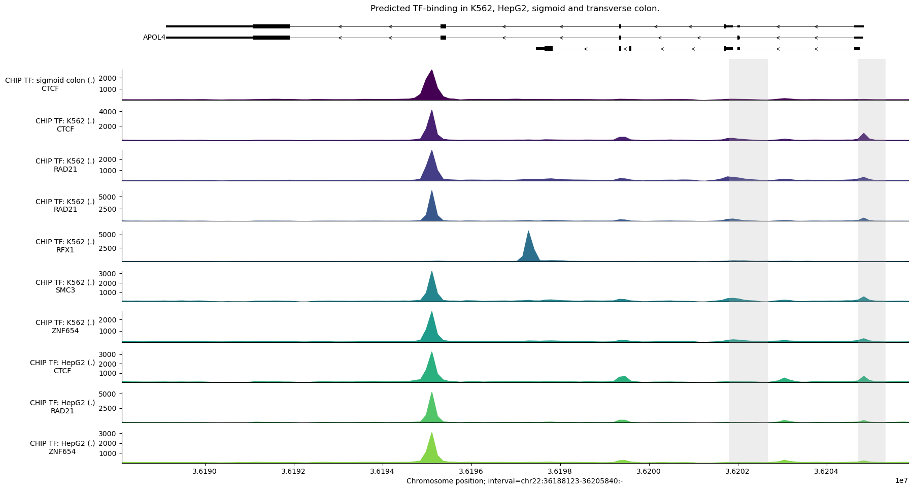
We observe a strong predicted CTCF peak near the second-to-last exon (counting from the right), which is predicted across different tissues.

We can average the signal for a transcription factor across tissues to simplify the plot. For example, to plot the mean CTCF signal across tissues, we first need to construct a new TrackData object:

mean_ctcf = output_filtered.values[
    :, output_filtered.metadata['transcription_factor'] == 'CTCF'
].mean(axis=1)

# Construct a new TrackData object from the mean values.
tdata_mean_ctcf = track_data.TrackData(
    values=mean_ctcf[:, None],
    metadata=pd.DataFrame(
        {'transcription_factor': ['CTCF'], 'name': ['mean'], 'strand': ['.']}
    ),
    interval=output_filtered.interval,
    resolution=output_filtered.resolution,
)

And then plot as usual:

plot_components.plot(
    [
        plot_components.TranscriptAnnotation(transcripts),
        plot_components.Tracks(
            tdata=tdata_mean_ctcf,
            ylabel_template='{name} {transcription_factor}',
            filled=True,
        ),
    ],
    interval=apol4_interval,
    annotations=[plot_components.IntervalAnnotation(promoter_intervals)],
    despine_keep_bottom=True,
    title='Predicted CTCF binding (mean across cell types)',
)
plt.show()

Contact maps

CONTACT_MAPS predicts 3D contact frequency between pairs of 2048 bp bins, normalized for distance decay (observed over expected, from Hi-C and Micro-C data). Use intervals substantially wider than 2048 bp.

Let’s make contact map predictions for a colon carcinoma cell line:

condition = 'EFO:0002824'  # HCT116 colon carcinoma cell line.

output = dna_model.predict_interval(
    interval=interval,
    requested_outputs={dna_client.OutputType.CONTACT_MAPS},
    condition=condition,
)

And plot the predicted DNA-DNA contacts:

plot = plot_components.plot(
    [
        plot_components.TranscriptAnnotation(longest_transcripts),
        plot_components.ContactMaps(
            tdata=output.contact_maps,
            ylabel_template='{biosample_name}\n{name}',
            cmap='autumn_r',
            vmax=2.0,
        ),
    ],
    interval=interval,
    title='Predicted contact maps',
)
plt.show()

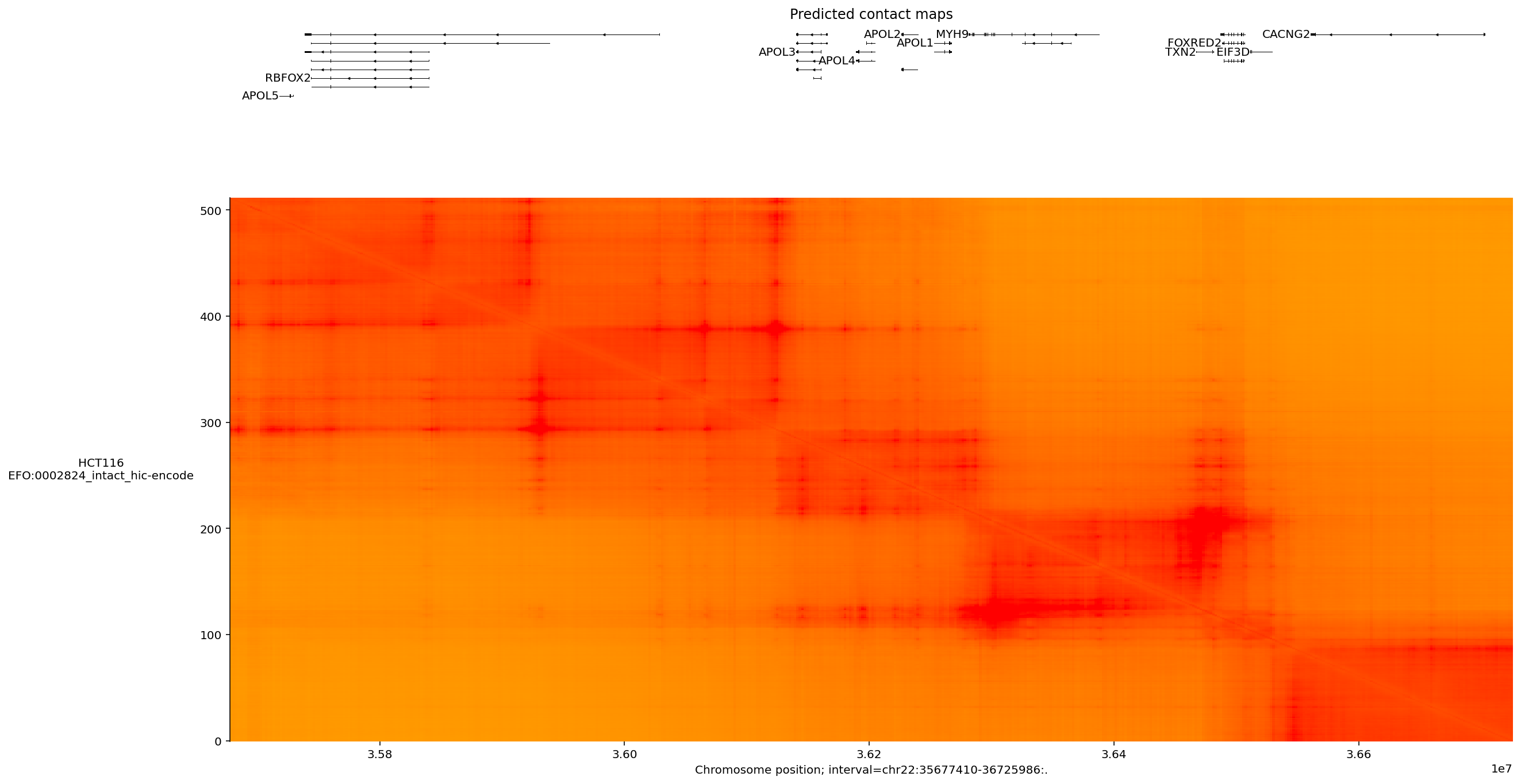
Several prominent interacting regions, potentially representing topologically-associated domains (TADs), are visible as blocks.